Random Numbers and Vectors from Multivariate Normal Distributions

Open Live Script

This example shows how to generate and visualize random numbers and vectors that are drawn from multivariate normal distributions. This example discusses the steps to generate and visualize random numbers and vectors that are drawn from univariate, bivariate, and trivariate normal distributions. The randn function generates random numbers from the standard normal distribution. To generate random numbers and vectors from a multivariate normal distribution with a specific mean and covariance, you can transform the data generated from the standard normal distribution. Starting from a $d$ -dimensional random variable $u = [u_{1}, u_{2}, . . ., u_{d}]$ that follows a normal distribution with zero mean and a unit covariance matrix, you can transform $u$ to $v = μ + u R$ . The variable $v$ follows the normal distribution with mean $μ$ and covariance matrix $Σ = R^{T} R$ . The covariance matrix $Σ$ is a symmetric and positive definite (nonsingular) matrix, which indicates that the multivariate normal distribution is also nondegenerate. Therefore, you can perform Cholesky decomposition on $Σ$ to obtain the upper triangular matrix $R$ . A multivariate normal distribution that is degenerate, where $Σ$ is not full rank (or singular), is beyond the scope of this example.

Univariate Normal Distribution

In statistics, a normal distribution, or Gaussian distribution, is a type of continuous probability distribution for a real random variable. The univariate normal distribution of the random variable $x$ is a probability density function (pdf) that has the form

$f (x) = \frac{1}{σ \sqrt{2 π}} \exp [- \frac{1}{2} {(\frac{x - μ}{σ})}^{2}]$ .

The parameter $μ$ is the mean of the distribution, and $σ$ is the standard deviation, with $σ^{2}$ being the variance of the distribution.

Standard Normal Distribution

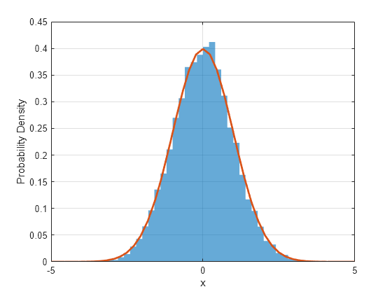
The simplest case of a normal distribution is the standard normal distribution, which has a mean of $μ = 0$ and a standard deviation of $σ = 1$ . In MATLAB®, you can use randn to generate random numbers that follow the standard normal distribution. For example, generate 10,000 random numbers.

n = 10000;
x_standard = randn(n,1);

Plot the probability density estimate of these numbers using histogram.

figure
histogram(x_standard,Normalization="pdf",EdgeColor="none")
xlabel("x")
ylabel("Probability Density")
grid on
hold on

To compare the sampled numbers with the pdf of the standard normal distribution, plot the pdf using fplot.

f = @(x) (1/sqrt(2*pi))*exp(-1/2*x.^2);
fplot(f,[-5 5],LineWidth=2)

Figure contains an axes object. The axes object with xlabel x, ylabel Probability Density contains 2 objects of type histogram, functionline.

Normal Distribution with Specified Mean and Standard Deviation

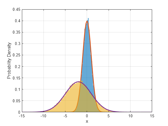
To generate random numbers from a univariate normal distribution with a specific mean $μ$ and standard deviation $σ$ , you can transform the data generated from the standard normal distribution by multiplying the data by $σ$ and adding $μ$ . For example, transform the previously generated random numbers so that they follow a normal distribution with a mean of $μ = - 2$ and a standard deviation of $σ = 3$ .

mu = -2;
sigma = 3;
x_transformed = sigma*x_standard + mu;

Calculate the mean and the standard deviation of the transformed data. The results do not exactly match the specified mean and standard deviation because the calculation from the sampling of the distribution determines these results.

mu_data = mean(x_transformed)

mu_data = 
-1.9950

sigma_data = std(x_transformed)

sigma_data = 
2.9744

Plot the probability density estimate and pdf of the transformed data.

histogram(x_transformed,Normalization="pdf",EdgeColor="none")
g = @(x) (1/(sigma*sqrt(2*pi)))*exp(-1/2*((x-mu)/sigma).^2);
fplot(g,[-15 15],LineWidth=2)
hold off

Figure contains an axes object. The axes object with xlabel x, ylabel Probability Density contains 4 objects of type histogram, functionline.

Multivariate Normal Distribution

The multivariate normal distribution extends the univariate normal distribution to two or more variables. It has two parameters: a mean vector $μ$ and a covariance matrix $Σ$ , which are analogous to the mean and variance parameters of a univariate normal distribution. In this example, the covariance matrix $Σ$ is restricted to being a symmetric and positive definite (nonsingular) matrix, indicating that the multivariate normal distribution is nondegenerate. The diagonal elements of $Σ$ contain the variances for each variable, and the off-diagonal elements of $Σ$ contain the covariances between variables.

The pdf of the $d$ -dimensional multivariate normal distribution is

$f (v_{1}, \dots, v_{d}) = \frac{\exp (- \frac{1}{2} (v - μ) Σ^{- 1} (v - μ)^{T})}{\sqrt{(2 π)^{d} | Σ |}},$

where $v$ and $μ$ are 1-by- $d$ row vectors, $Σ$ is a $d$ -by- $d$ symmetric, positive definite matrix, and $| Σ |$ is the determinant of $Σ$ .

Bivariate Normal Distribution with Zero Mean and Unit Covariance

In the two-dimensional case, the multivariate normal distribution becomes a bivariate normal distribution, which can also be written as

$f (x, y) = \frac{1}{2 π σ_{x} σ_{y} \sqrt{1 - ρ_{x y}^{2}}} \exp (- \frac{1}{2 (1 - ρ_{x y}^{2})} [{(\frac{x - μ_{x}}{σ_{x}})}^{2} - 2 ρ_{x y} (\frac{x - μ_{x}}{σ_{x}}) (\frac{y - μ_{y}}{σ_{y}}) + {(\frac{y - μ_{y}}{σ_{y}})}^{2}]),$

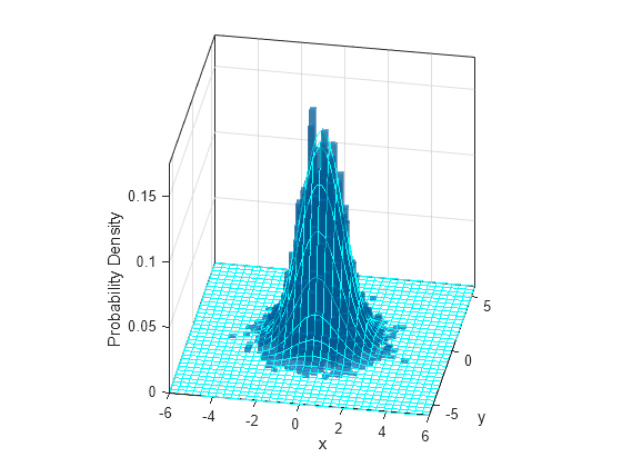
where the standard deviation of $x$ is $σ_{x} > 0$ , the standard deviation of $y$ is $σ_{y} > 0$ , and the correlation coefficient between the random variables $x$ and $y$ is $- 1 < ρ_{x y} < 1$ . In this case, the mean vector is $μ = [μ_{x}, μ_{y}]$ . The covariance matrix is $Σ = [\begin{array}{c} σ_{x}^{2} & ρ_{x y} σ_{x} σ_{y} \\ ρ_{x y} σ_{x} σ_{y} & σ_{y}^{2} \end{array}]$ .

If $σ_{x} = σ_{y}$ and $ρ_{x y} = 0$ , then the bivariate normal distribution is a circularly symmetric bell-shaped surface in the $x y$ -plane that is centered at $μ$ .

For the special case where $x$ and $y$ are independent random variables that follow the standard normal distribution, the mean vector of the bivariate distribution is 0 and the covariance matrix is a 2-by-2 identity matrix. To generate random vectors that follow this bivariate normal distribution, you can use randn directly without any transformation. For example, generate 10,000 data points of 1-by-2 random vectors by specifying the array size when using randn. Plot the 2-D probability density estimate of these bivariate random vectors using histogram2. To compare the sampled vectors with the pdf of the bivariate normal distribution, plot the pdf using fmesh.

u = randn(n,2);

figure
histogram2(u(:,1),u(:,2),Normalization="pdf",FaceAlpha=0.5,EdgeColor="none")
xlabel("x")
ylabel("y")
zlabel("Probability Density")
axis([-6 6 -6 6])
axis square
view(10,30)
hold on

mu = [0 0];
sigma = [1 0; 0 1];
f = @(x,y) exp(-0.5*dot(([x(:),y(:)]-mu),(sigma\([x(:),y(:)]-mu)')',2)')/ ...
    sqrt((2*pi)^2*det(sigma));
fmesh(f,FaceAlpha=0,EdgeColor="cyan")
hold off

Figure contains an axes object. The axes object with xlabel x, ylabel y contains 2 objects of type histogram2, functionsurface.

Bivariate Normal Distribution with Specified Mean and Covariance Matrix

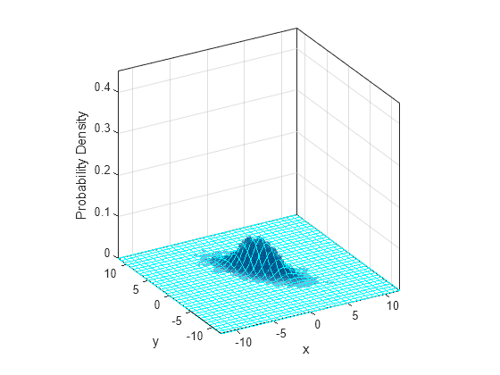
To generate random vectors from a general bivariate normal distribution with a specific mean and covariance, you need to transform the previously generated data. Starting from a $d$ -dimensional random variable $u = [u_{1}, u_{2}, . . ., u_{d}]$ that follows a normal distribution with zero mean and unit covariance matrix, you can transform $u$ to $v = μ + u R$ . The variable $v$ follows the normal distribution with mean $μ$ and covariance matrix $Σ = R^{T} R$ .

For example, specify the mean as $μ = [0.5, 1]$ . Specify the standard deviation of $x$ as $σ_{x} = 1.4$ , the standard deviation to $y$ as $σ_{y} = 2$ , and the correlation coefficient to $ρ_{x y} = - 0.7$ . The covariance matrix becomes $Σ = [\begin{array}{c} σ_{x}^{2} & ρ_{x y} σ_{x} σ_{y} \\ ρ_{x y} σ_{x} σ_{y} & σ_{y}^{2} \end{array}] = [\begin{array}{c} 1.96 & - 1.96 \\ - 1.96 & 4 \end{array}]$ .

To interactively change the values of $σ_{x}$ , $σ_{y}$ , and $ρ_{x y}$ , you can add sliders to your script. Go to the Insert tab, click the Control button, and select Slider. For more information, see Add Interactive Controls to a Live Script. Add three interactive sliders that set the values of $σ_{x}$ , $σ_{y}$ , and $ρ_{x y}$ . By default, when these values change, the Live Editor only runs the code in the current section. Configure this behavior by right-clicking the sliders, selecting Configure Control, and setting Run in the Execution section to Current section to end. This ensures the code in the section containing the sliders and any following sections runs whenever the values of the sliders change.

mu = [0.5 1];
sigma_x = 1.4;
sigma_y = 2;
rho_xy = -0.7;
sigma = [sigma_x^2,              rho_xy*sigma_x*sigma_y;
         rho_xy*sigma_x*sigma_y, sigma_y^2 ];

Perform the Cholesky decomposition of the covariance matrix. The result is an upper triangular matrix $R$ such that $Σ = R^{T} R$ . Scale the original data by this matrix and shift the scaled data to the specified mean.

R = chol(sigma);
v = mu + u*R;

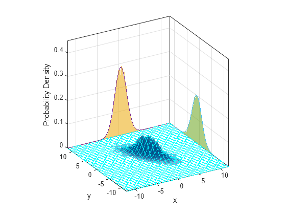
Plot the 2-D probability density estimate of the transformed data using histogram2. To compare the sampled vectors with the pdf of the bivariate normal distribution, plot the pdf using fmesh.

figure
histogram2(v(:,1),v(:,2),Normalization="pdf",FaceAlpha=0.5,EdgeColor="none")
xlabel("x")
ylabel("y")
zlabel("Probability Density")
axis([-12 12 -12 12 0 0.45])
axis square
view(330,25)
hold on

f = @(x,y) exp(-0.5*dot(([x(:),y(:)]-mu),(sigma\([x(:),y(:)]-mu)')',2)')/ ...
    sqrt((2*pi)^2*det(sigma));
fmesh(f,FaceAlpha=0,EdgeColor="cyan")

Figure contains an axes object. The axes object with xlabel x, ylabel y contains 2 objects of type histogram2, functionsurface.

Marginal Distributions of Bivariate Normal Distribution

One property of a multivariate normal distribution is that the marginal distribution of any subset of the random variables is also a multivariate normal distribution corresponding to that subset. In other words, the marginal distribution of $x$ from the bivariate normal distribution $f (x, y)$ is a univariate normal distribution $f_{x} (x)$ with $μ_{x}$ as its mean and $σ_{x}$ as its standard deviation, which can be written as

$f_{x} (x) = \int_{- \infty}^{\infty} f (x, y) dy = \frac{1}{σ_{x} \sqrt{2 π}} \exp [- \frac{1}{2} {(\frac{x - μ_{x}}{σ_{x}})}^{2}]$ .

The marginal distribution of $y$ from the bivariate normal distribution $f (x, y)$ is a univariate normal distribution $f_{y} (y)$ with $μ_{y}$ as its mean and $σ_{y}$ as its standard deviation. In the case of the bivariate normal distribution, changing the correlation coefficient $ρ_{x y}$ does not affect the marginal distribution of $x$ or $y$ .

To show this property, you can plot the marginal distributions of the transformed data in the previous section. Plot the marginal distribution of $x$ by using histogram on v(:,1). For visualization purposes, plot this distribution in the ( $x$ ,pdf)-plane by using hgtransform and applying rotation and translation transformations to bring the plot into the plane. Compare the marginal distribution of $x$ with the pdf of the univariate normal distribution using fplot.

ax = gca;
hgx = hgtransform(ax);
hgx.Matrix = makehgtform("xrotate",pi/2,"translate",[0 0 -12]);
histogram(v(:,1),Normalization="pdf",EdgeColor="none",Parent=hgx)

f = @(x) exp(-0.5*(x-mu(1)).^2/sigma(1,1))/sqrt((2*pi)*sigma(1,1));
fplot(f,[-12 12],Parent=hgx)

Plot the marginal distribution of $y$ by using histogram on v(:,2). Plot this distribution in the ( $y$ ,pdf)-plane. Compare the marginal distribution of $y$ with the pdf of the univariate normal distribution using fplot.

hgy = hgtransform(ax);
hgy.Matrix = makehgtform("xrotate",pi/2,"yrotate",pi/2,"translate",[0 0 12]);
histogram(v(:,2),Normalization="pdf",EdgeColor="none",Parent=hgy)

f = @(y) exp(-0.5*(y-mu(2)).^2/sigma(2,2))/sqrt((2*pi)*sigma(2,2));
fplot(f,[-12 12],Parent=hgy)
hold off;

Figure contains an axes object. The axes object with xlabel x, ylabel y contains 6 objects of type histogram, functionline, histogram2, functionsurface.

Trivariate Normal Distribution

To generate random vectors from any nondegenerate multivariate normal distribution, you can follow the steps outlined in previous sections. For example, generate random vectors from a trivariate normal distribution with a specific mean and covariance matrix. Specify the mean as $μ = [μ_{x}, μ_{y}, μ_{z}] = [1, 1.5, - 1.5]$ . Specify the covariance matrix as $Σ = [\begin{array}{c} σ_{x}^{2} & σ_{x y} & σ_{x z} \\ σ_{x y} & σ_{y}^{2} & σ_{y z} \\ σ_{x z} & σ_{y z} & σ_{z}^{2} \end{array}] = [\begin{array}{c} 2 & - 1.5 & 0.5 \\ - 1.5 & 4 & 2 \\ 0.5 & 2 & 3 \end{array}]$ .

Because there are three random variables, generate 10,000 data points of 1-by-3 random vectors from the standard normal distribution by specifying the array size when using randn. Apply the transformation so that the generated data follows the specified multivariate normal distribution.

u_3D = randn(n,3);
mu = [1 1.5 -1.5];
sigma = [2 -1.5 0.5; -1.5 4 2; 0.5 2 3];
R = chol(sigma);
v = mu + u_3D*R;

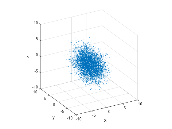
Because the data already consists of 3-D points, you cannot visualize the histogram of the probability density in 3-D space (you would need an additional axis to show the frequencies). Instead, you can plot the location of the 3-D points by using scatter3.

figure
scatter3(v(:,1),v(:,2),v(:,3),1,".")
axis([-10 10 -10 10 -10 10])
axis square
xlabel("x")
ylabel("y")
zlabel("z")
grid on
view(330,25)

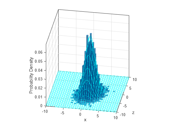
Figure contains an axes object. The axes object with xlabel x, ylabel y contains an object of type scatter.

You can also check if the generated data satisfies the property of the marginal distribution of a multivariate normal distribution. For example, the marginal distribution of $(x, z)$ is a bivariate normal distribution with the mean $μ = [μ_{x}, μ_{z}]$ and the covariance matrix $Σ = [\begin{array}{c} σ_{x}^{2} & σ_{x z} \\ σ_{x z} & σ_{z}^{2} \end{array}]$ .

Plot the marginal distribution of $(x, z)$ by using histogram2 on v(:,1) and v(:,3). Compare the marginal distribution of $(x, z)$ with the pdf of the bivariate normal distribution using fmesh.

figure
histogram2(v(:,1),v(:,3),Normalization="pdf",FaceAlpha=0.5,EdgeColor="none")
xlabel("x")
ylabel("z")
zlabel("Probability Density")
axis([-10 10 -10 10])
axis square
view(10,30)
hold on

fxz = @(x,z) exp(-0.5*dot(([x(:),z(:)]-mu([1 3])),(sigma([1 3],[1 3])\ ...
      ([x(:),z(:)]-mu([1 3]))')',2)')/sqrt((2*pi)^2*det(sigma([1 3],[1 3])));
fmesh(fxz,FaceAlpha=0,EdgeColor="cyan")
hold off

Figure contains an axes object. The axes object with xlabel x, ylabel z contains 2 objects of type histogram2, functionsurface.