主要内容

本页翻译不是最新的。点击此处可查看最新英文版本。

makima

修正 Akima 分段三次 Hermite 插值

说明

yq = makima(x,y,xq) 使用采样点 x 处的值 y 执行修正 Akima 插值,以求出查询点 xq 处的插值 yq

示例

pp = makima(x,y) 返回一个分段多项式结构体以用于 ppval 和样条实用工具 unmkpp

示例

示例

全部折叠

使用 makima 对非等间距采样点上的余弦曲线进行插值。

x = [0 1 2.5 3.6 5 7 8.1 10];
y = cos(x);
xq = 0:.25:10;
yq = makima(x,y,xq);
plot(x,y,'o',xq,yq,'--')

Figure contains an axes object. The axes object contains 2 objects of type line. One or more of the lines displays its values using only markers

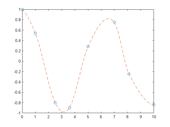
Akima 算法利用振荡函数使局部极值附近的曲线展平。为了补偿这种展平,您可以在局部极值附近添加更多采样点。
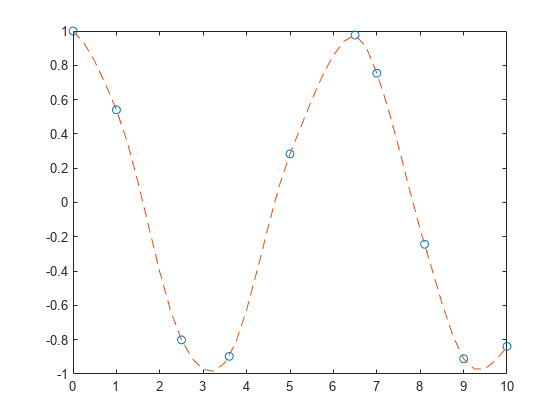
x=6.5x=9 附近添加采样点,然后重新绘制插值。

x = [0 1 2.5 3.6 5 6.5 7 8.1 9 10];
y = cos(x);
xq = 0:.25:10;
yq = makima(x,y,xq);
plot(x,y,'o',xq,yq,'--')

Figure contains an axes object. The axes object contains 2 objects of type line. One or more of the lines displays its values using only markers

splinepchipmakima 为两个不同数据集生成的插值结果进行比较。这些函数都执行不同形式的分段三次 Hermite 插值。每个函数计算插值斜率的方式不同,因此它们在基础数据的平台区或波动处展现出不同行为。

对连接两个平台区的样本数据进行插值,并比较结果。创建由 x 值、点 y 处的函数值以及查询点 xq 组成的向量。使用 splinepchipmakima 计算查询点处的插值。绘制查询点处的插值函数值以进行比较。

x = -3:3; 
y = [-1 -1 -1 0 1 1 1]; 
xq1 = -3:.01:3;
p = pchip(x,y,xq1);
s = spline(x,y,xq1);
m = makima(x,y,xq1);
plot(x,y,'o',xq1,p,'-',xq1,s,'-.',xq1,m,'--')
legend('Sample Points','pchip','spline','makima','Location','SouthEast')
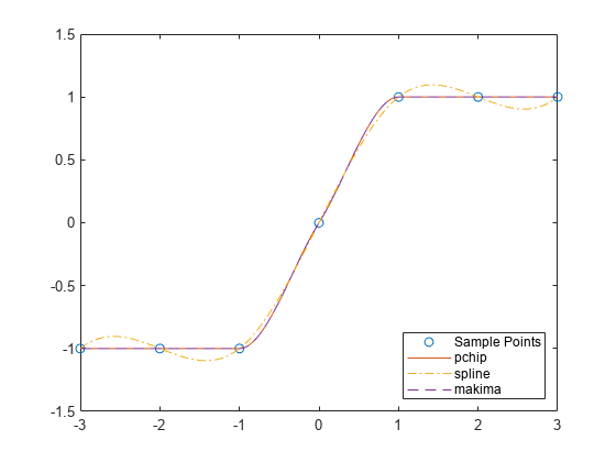
Figure contains an axes object. The axes object contains 4 objects of type line. One or more of the lines displays its values using only markers These objects represent Sample Points, pchip, spline, makima.

在本例中,pchipmakima 具有相似的行为,因为它们可以避免过冲,并且可以准确地连接平台区。

使用振动采样函数执行第二次比较。

x = 0:15;
y = besselj(1,x);
xq2 = 0:0.01:15;
p = pchip(x,y,xq2);
s = spline(x,y,xq2);
m = makima(x,y,xq2);
plot(x,y,'o',xq2,p,'-',xq2,s,'-.',xq2,m,'--')
legend('Sample Points','pchip','spline','makima')
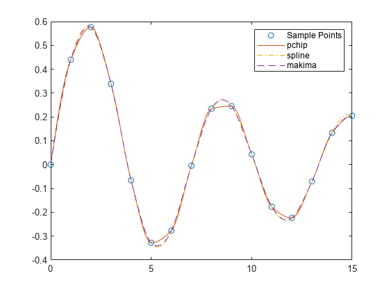
Figure contains an axes object. The axes object contains 4 objects of type line. One or more of the lines displays its values using only markers These objects represent Sample Points, pchip, spline, makima.

当基础函数振荡时,splinemakima 能够比 pchip 更好地捕获点之间的移动,后者会在局部极值附近急剧展平。

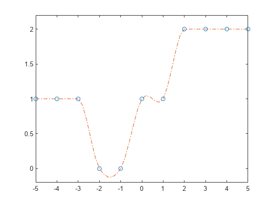
创建采样点 x 及其值 y 的向量。使用 makima 为数据构造一个分段多项式结构体。

x = -5:5;
y = [1 1 1 0 0 1 1 2 2 2 2];
pp = makima(x,y)
pp = struct with fields:
      form: 'pp'
    breaks: [-5 -4 -3 -2 -1 0 1 2 3 4 5]
     coefs: [10×4 double]
    pieces: 10
     order: 4
       dim: 1

该结构体包含涵盖整个数据的 10 个 4 阶多项式的信息。pp.coefs(i,:) 包含在断点 [breaks(i) breaks(i+1)] 定义的区域内有效的多项式的系数。

结合 ppval 使用该结构体以计算几个查询点处的插值,然后绘制结果。在有三个或更多连续等值点的区域,Akima 算法用直线将这些点连接起来。

xq = -5:0.2:5;
m = ppval(pp,xq);
plot(x,y,'o',xq,m,'-.')
ylim([-0.2 2.2])

Figure contains an axes object. The axes object contains 2 objects of type line. One or more of the lines displays its values using only markers

输入参数

全部折叠

样本点,指定为一个向量。向量 x 指定提供数据 y 的点。x 的元素必须是唯一的。

数据类型: single | double

样本点处的函数值,指定为数值向量、矩阵或数组。xy 的长度必须相同。

如果 y 是矩阵或数组,则在获取最后一个维度 y(:,...,:,j) 中的值时应使其匹配 x。在此情况下,y 的最后一个维度的长度必须与 x 相同。

数据类型: single | double

查询点,指定为标量、向量、矩阵或数组。xq 中指定的点是 makima 计算出的插值函数值 yqx 坐标。

数据类型: single | double

输出参量

全部折叠

查询点处的插值,以标量、向量、矩阵或数组形式返回。yq 的大小与 yxq 的大小相关:

  • 如果 y 为向量,则 yq 的大小与 xq 相同。

  • 如果 y 是大小为 Ny = size(y) 的数组,则下列条件适用:

    • 如果 xq 为标量或向量,则 size(yq) 返回 [Ny(1:end-1) length(xq)]

    • 如果 xq 是数组,则 size(yq) 返回 [Ny(1:end-1) size(xq)]

分段多项式,以结构体形式返回。将此结构体与 ppval 函数结合使用可计算一个或多个查询点处的插值多项式。该结构体包含以下字段。

字段描述
form

'pp'分段多项式

breaks

包含严格递增元素的长度为 L+1 的向量,这些元素代表 L 个区间中每个区间的开始点和结束点

coefs

L×k 矩阵,其中每行 coefs(i,:) 包含第 i 个区间 [breaks(i),breaks(i+1)]k 次多项式的局部系数

pieces

段数 L

order

多项式的阶

dim

目标的维度

由于 coefs 中的多项式系数是每个区间的本地系数,因此您必须减去对应节点区间的较低端点,以使用传统多项式方程中的系数。换言之,对于区间 [x1,x2] 上的系数 [a,b,c,d],对应的多项式为

f(x)=a(xx1)3+b(xx1)2+c(xx1)+d.

详细信息

全部折叠

参考

[1] Akima, Hiroshi. "A new method of interpolation and smooth curve fitting based on local procedures." Journal of the ACM (JACM) , 17.4, 1970, pp. 589–602.

[2] Akima, Hiroshi. "A method of bivariate interpolation and smooth surface fitting based on local procedures." Communications of the ACM , 17.1, 1974, pp. 18–20.

扩展功能

全部展开

版本历史记录

在 R2019b 中推出