Main Content

makima

Modified Akima piecewise cubic Hermite interpolation

Since R2019b

Description

example

yq = makima(x,y,xq) performs Modified Akima Interpolation using the values y at sample points x to find interpolated values yq at the query points xq.

example

pp = makima(x,y) returns a piecewise polynomial structure for use with ppval and the spline utility unmkpp.

Examples

collapse all

Use makima to interpolate a cosine curve over unevenly spaced sample points.

x = [0 1 2.5 3.6 5 7 8.1 10];
y = cos(x);
xq = 0:.25:10;
yq = makima(x,y,xq);
plot(x,y,'o',xq,yq,'--')

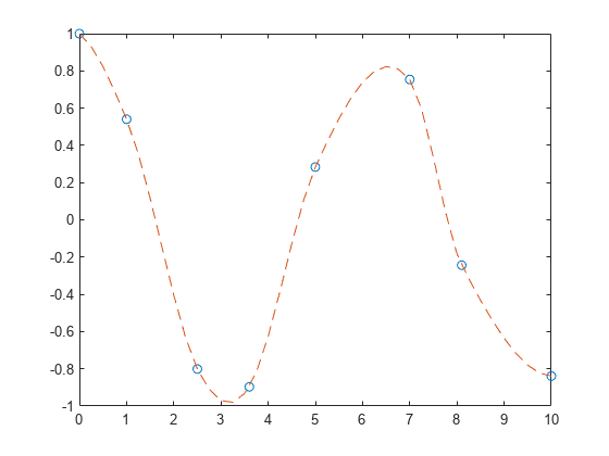
With oscillatory functions, the Akima algorithm flattens the curve near local extrema. To compensate for this flattening, you can add more sample points near the local extrema.
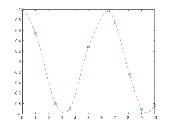
Add sample points near x=6.5 and x=9 and replot the interpolation.

x = [0 1 2.5 3.6 5 6.5 7 8.1 9 10];
y = cos(x);
xq = 0:.25:10;
yq = makima(x,y,xq);
plot(x,y,'o',xq,yq,'--')

Compare the interpolation results produced by spline, pchip, and makima for two different data sets. These functions all perform different forms of piecewise cubic Hermite interpolation. Each function differs in how it computes the slopes of the interpolant, leading to different behaviors when the underlying data has flat areas or undulations.

Compare the interpolation results on sample data that connects flat regions. Create vectors of x values, function values at those points y, and query points xq. Compute interpolations at the query points using spline, pchip, and makima. Plot the interpolated function values at the query points for comparison.

x = -3:3; 
y = [-1 -1 -1 0 1 1 1]; 
xq1 = -3:.01:3;
p = pchip(x,y,xq1);
s = spline(x,y,xq1);
m = makima(x,y,xq1);
plot(x,y,'o',xq1,p,'-',xq1,s,'-.',xq1,m,'--')
legend('Sample Points','pchip','spline','makima','Location','SouthEast')

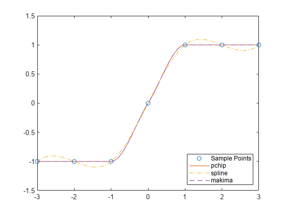
In this case, pchip and makima have similar behavior in that they avoid overshoots and can accurately connect the flat regions.

Perform a second comparison using an oscillatory sample function.

x = 0:15;
y = besselj(1,x);
xq2 = 0:0.01:15;
p = pchip(x,y,xq2);
s = spline(x,y,xq2);
m = makima(x,y,xq2);
plot(x,y,'o',xq2,p,'-',xq2,s,'-.',xq2,m,'--')
legend('Sample Points','pchip','spline','makima')

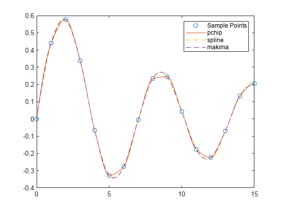
When the underlying function is oscillatory, spline and makima capture the movement between points better than pchip, which is aggressively flattened near local extrema.

Create vectors for the sample points x and values at those points y. Use makima to construct a piecewise polynomial structure for the data.

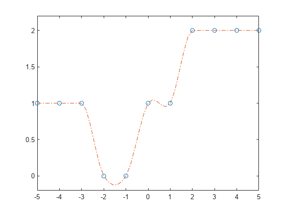
x = -5:5;
y = [1 1 1 0 0 1 1 2 2 2 2];
pp = makima(x,y)
pp = struct with fields:
      form: 'pp'
    breaks: [-5 -4 -3 -2 -1 0 1 2 3 4 5]
     coefs: [10x4 double]
    pieces: 10
     order: 4
       dim: 1

The structure contains the information for 10 polynomials of order 4 that span the data. pp.coefs(i,:) contains the coefficients for the polynomial that is valid in the region defined by the breakpoints [breaks(i) breaks(i+1)].

Use the structure with ppval to evaluate the interpolation at several query points, and then plot the results. In regions with three or more constant points, the Akima algorithm connects the points with a straight line.

xq = -5:0.2:5;
m = ppval(pp,xq);
plot(x,y,'o',xq,m,'-.')
ylim([-0.2 2.2])

Input Arguments

collapse all

Sample points, specified as a vector. The vector x specifies the points at which the data y is given. The elements of x must be unique.

Data Types: single | double

Function values at sample points, specified as a numeric vector, matrix, or array. x and y must have the same length.

If y is a matrix or array, then the values in the last dimension, y(:,...,:,j), are taken as the values to match with x. In that case, the last dimension of y must be the same length as x.

Data Types: single | double

Query points, specified as a scalar, vector, matrix, or array. The points specified in xq are the x-coordinates for the interpolated function values yq computed by makima.

Data Types: single | double

Output Arguments

collapse all

Interpolated values at query points, returned as a scalar, vector, matrix, or array. The size of yq is related to the sizes of y and xq:

  • If y is a vector, then yq has the same size as xq.

  • If y is an array of size Ny = size(y), then these conditions apply:

    • If xq is a scalar or vector, then size(yq) returns [Ny(1:end-1) length(xq)].

    • If xq is an array, then size(yq) returns [Ny(1:end-1) size(xq)].

Piecewise polynomial, returned as a structure. Use this structure with the ppval function to evaluate the interpolating polynomials at one or more query points. The structure has these fields.

FieldDescription
form

'pp' for piecewise polynomial

breaks

Vector of length L+1 with strictly increasing elements that represent the start and end of each of L intervals

coefs

L-by-k matrix with each row coefs(i,:) containing the local coefficients of an order k polynomial on the ith interval, [breaks(i),breaks(i+1)]

pieces

Number of pieces, L

order

Order of polynomials

dim

Dimensionality of target

Because the polynomial coefficients in coefs are local coefficients for each interval, you must subtract the lower endpoint of the corresponding knot interval to use the coefficients in a conventional polynomial equation. In other words, for the coefficients [a,b,c,d] on the interval [x1,x2], the corresponding polynomial is

f(x)=a(xx1)3+b(xx1)2+c(xx1)+d.

More About

collapse all

Modified Akima Interpolation

The Akima algorithm for one-dimensional interpolation, described in [1] and [2], performs cubic interpolation to produce piecewise polynomials with continuous first-order derivatives (C1). The algorithm avoids excessive local undulations.

If δi=vi+1vixi+1xi is the slope on interval [xixi+1), then the value of the derivative di at the sample point xi is a weighted average of nearby slopes:

di=w1w1+w2δi1+w2w1+w2δi.

In Akima's original formula, the weights are:

w1=|δi+1δi|,w2=|δi1δi2|.

The original Akima algorithm gives equal weight to the points on both sides, evenly dividing an undulation.

When two flat regions with different slopes meet, the modification made to the original Akima algorithm gives more weight to the side where the slope is closer to zero. This modification gives priority to the side that is closer to horizontal, which is more intuitive and avoids overshoot. In particular, whenever there are three or more consecutive collinear points, the algorithm connects them with a straight line and thus avoids an overshoot.

The weights used in the modified Akima algorithm are:

w1=|δi+1δi|+|δi+1+δi|2,w2=|δi1δi2|+|δi1+δi2|2.

Compared to the spline algorithm, the Akima algorithm produces fewer undulations and is better suited to deal with quick changes between flat regions. Compared to the pchip algorithm, the Akima algorithm is not as aggressively flattened and is therefore still able to deal with oscillatory data.

References

[1] Akima, Hiroshi. "A new method of interpolation and smooth curve fitting based on local procedures." Journal of the ACM (JACM) , 17.4, 1970, pp. 589–602.

[2] Akima, Hiroshi. "A method of bivariate interpolation and smooth surface fitting based on local procedures." Communications of the ACM , 17.1, 1974, pp. 18–20.

Extended Capabilities

Version History

Introduced in R2019b