Optimize Calibrations with Transient Controllers

Use the transient feature fill to optimize calibrations with transient controllers, enabling calibration of dynamic systems like diesel particulate filter (DPF) and nitric oxide and nitrogen dioxide (NOx) emission controllers and on-board diagnostics (OBD) estimators. Specifically, CAGE can optimize calibrations for transients features that:

Include delays, discrete integrators and filters, and feedback loops.
Contain many ( > 50) lookup tables that require calibration with transient data.
Have multiple test data files to tune the feature.
Require analytic derivatives to perform large-scale optimizations.

For large feature fills, the fill can take a long time to run. If it is available, CAGE uses the Parallel Computing Toolbox™ to evaluate calibration data files on different workers.

To use the transient feature fill, follow these workflow steps.

Step		Description
1	Import Simulink Model	Use CAGE to import the Simulink^® model that has the transient features.
2	Run Optimization	Use the Feature Fill Wizard to specify the fill settings and run the optimization.
3	Restart Optimization	Optionally, stop and restart the optimization.
4	Analyze Results	Use CAGE to analyze the optimization results.
5	Export Calibration	Export the tables in calibration formats, including `INCA DCM` and `CSV` file formats.

Import Simulink Model

Use CAGE to import the Simulink model that has the transient features.

In CAGE, select File > Import > Strategy. Use the browser to select the Simulink model with the transient features.
Use the MBC Feature Importer to preview lookup tables and import features for selected Simulink subsystems. Click OK.
If you import a Simulink model with a transient block, the CAGE Parser dialog box prompts you to set the data sample rate.
For data with a constant sample rate, the rate should allow the Simulink model to run with an ode1 solver. Typically, this sample time is about 0.1s to 1s.
For data with a variable sample rate, set the value to -1 or 0.
- The data file must contain a signal named time. After you import the strategy, you can use the CAGE variable dictionary to rename the time signal.
- To calculate the sample time, CAGE uses a discrete filter.
- Battery characterization tests can have variable same rates.. The tests are long running and consist of a transient response requiring a fast sample time (0.01 to 0.1s), followed by near steady-state conditions which are sampled at a lower rate.
For information about block support in CAGE, see Block Support.

Run Optimization

Before you start, make sure that you have the statistical response model aligned with the feature inputs. For more information, see Set Up Models for Calibration and Set Up Variables and Constants.

To run the optimization, in CAGE, click Feature Filling . Use the Feature Fill Wizard to specify the fill settings.

Select Feature > Fill Feature.
In the Feature Fill Wizard, select Use large scale feature fill.
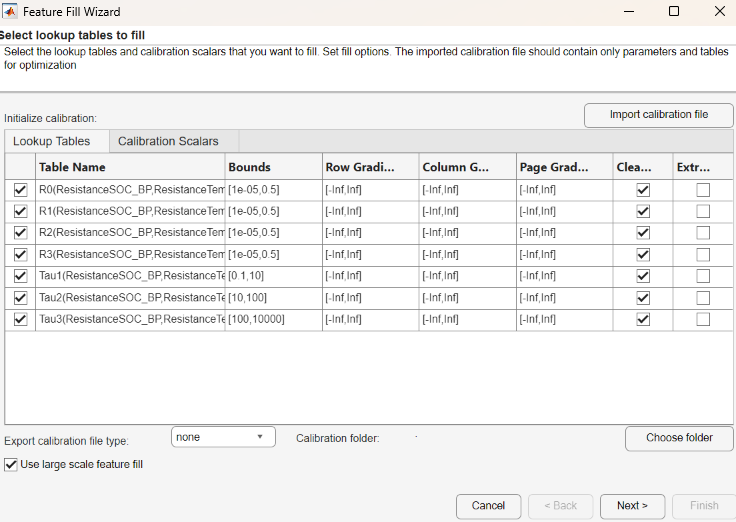
- On the Lookup Tables tab, select all of the tables.
- On the Calibration Scalars tab, select the calibration constraints that you want to use in the optimization. Starting from R2024a, the nonlinear least-squares algorithm supports gradient constraints for large-scale optimizations.
- To specify a calibration data file that optimizes and initializes the lookup tables and scalars, select Import calibration file. Make sure that the calibration file contains only parameters and table that you want to use in the optimization. The file must be one of the supported formats listed in Import and Export Calibrations.
- If you are characterizing battery block parameters and choose to automatically update the Simulink parameters when the feature fill completes, Simulink Block is selected for Export calibration file type.
Click Next.

In the wizard, specify the data folder, signals, and initial conditions.

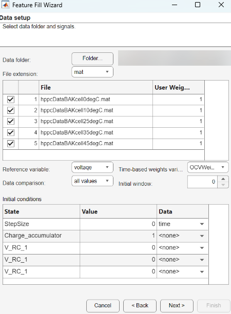
Image showing feature fill wizard with optimization settings

Parameter	Description
Data folder	Folder containing test data and the file extension. The extension is either `CSV`, `xlsx`, or `mat`. MAT files must contain `table` objects or `timetable` objects. After you specify the folder and extension, CAGE finds compatible files. To be compatible, each file must contain all the feature inputs and a common additional column for the software to use to match against the feature. If CAGE is unable to locate files with the specified extension, it will search for and list files with other valid extensions instead. Uncheck the boxes for files you want to exclude, alternatively you can set the User Weights to zero for files you want to exclude.
File extension
Reference variable	Select the reference signal to compare to values in the data set.
Data comparison	Set parameter to compare `all values` or the `final value` in the data set to a reference signal.
User Weights	Specify a weight for each data set. This method defines the relevance of each data set in filling. Weights must be nonnegative values.
Time-based weights variable	Specify a time-based weight variable in the data set. This method defines the relevance for different segments of the data set in filling. For example, by using a time-based weight, you can either place more emphasis on different regions of the time series or exclude part of a time series by setting the weights variable to zero for that region. For an example calculating time-based weights, see Preprocess Battery Data and Initialize Battery Block Parameters for Feature Filling. Weights must be nonnegative values.
Initial window	Number of initial samples that CAGE ignores when comparing all values. Alternatively, if you have a weight variable available in the data file, you can set time-based weights to exclude initial samples. This approach offers more flexibility.
Initial conditions	Set the initial conditions for states, either: Value – Constant value Data – First specified signal value in data file

Click Next.

In the wizard, specify the Large scale Feature Fill optimization settings.

Image showing feature fill wizard with optimization settings

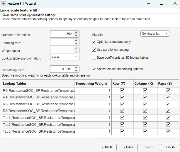
Parameter	Description
Number of iterations	Specify the Number of iterations.
Learning rate	Specify a Learning rate parameter for the `ADAM` algorithm. If you select the least squares algorithm, the Learning rate parameter corresponds to the step size.
Weight factor	Weighting factor for each test file, the default value is `1`. CAGE provides tests with a higher than average error a higher weight. In the case of matching all values, the weighting factor is inversely proportional to the number of observations in the test. If you specify user-defined weights, do not use a weight factor. It is recommended to set user-defined weights instead of a weight factor.
Lookup table approximation	Optimize lookup tables using linear, spline, or Chebyshev polynomials rather than using the lookup table values. `linear` (default) – Linear interpolation method. Consider using for optimizing ECU lookup tables. `spline` – Cubic spline interpolation method. Consider using for optimizing ECU lookup tables or lookup tables that are part of system simulations where smooth response surfaces are required. `chebyshev` – Chebyshev polynomials represent the lookup tables being optimized with fewer parameters than the lookup table cells. This type of optimization is useful when filling many (and possibly large) lookup tables. Use Chebyshev polynomials to start the filling process and switch to filling directly with lookup table values for the last stage.
Smoothing factor	CAGE applies a smoothing factor to the tables in the feature fill during the optimization. The smoothness penalty uses second differences to avoid steep jumps between adjacent table values. This parameter may need to be adjusted to achieve a smoother or less smooth lookup table. This smoothing factor acts as a filter against noisy data.
Algorithm	`Nonlinear least squares` (default) – Similar to the trust-region reflective algorithm used in the Optimization Toolbox™ `lsqnonlin` function. If you have table gradient constraints defined, the optimizer will use `fmincon`. This algorithm provides faster convergence. Use when the table values are close to the optimal values. `Nonlinear least squares (fmincon)` – The optimizer uses `fmincon` by default. This algorithm provides faster convergence. Use this option when there are gradient constraints. `ADAM` – Typically more robust in the initial search for an optimization solution. Use for large optimization problems with large data sets and many parameters. The algorithm is widely used in deep learning applications. For more information, see `trainingOptions` (Deep Learning Toolbox). `Eigenvalue analysis-based optimization scheme` – Faster convergence of second-order optimization terms. Use for feature fills that have many lookup tables to fill, when the `ADAM` algorithm has poor convergence and the default `Nonlinear least squares` algorithm is slow. `Analytic Hessian (slow)` – Consider using this method if the other methods fail to find a satisfactory solution. Although this option can be significantly slower than other methods, it can converge on a solution when other methods fail. This method is useful when the initial lookup table values are not close to the optimal solution. You may need a combination of different methods to obtain a solution. Start with the `ADAM` method.
Optimize simultaneously	For `Least squares` optimizations, select to account for lookup table couplings. Selecting this option might produce more accurate optimizations but slow performance.
Use parallel computing	Option to use parallel computing if you have a Parallel Computing Toolbox license. Different files are processed by separate workers.
Save coefficients as 1D lookup tables	Save coefficients of splines and Chebyshev polynomials as 1D lookup tables for visual inspections and export to `CSV` files.
Show detailed smoothing options	Specify Smoothing Weight to control smoothness for each lookup table. Disable smoothing for a lookup table by specifying Smoothing Weight as `0` or deselect a box to disable smoothing for a specific dimension. Smoothing weights are relative and indicate the importance of smoothness for each table. All weights are multiplied by the scalar smoothing factor.

Click Finish. As the feature fill runs, you can:
- Update the lookup table breakpoints if the test data covers less than half the table data.
- View progress in the Fill Progress dialog box.
  - Top plot displays fit for each file in the current iteration compared to previous iteration.
  - Bottom plot shows the improvement in RMSE over each iteration.
  - Use Lookup Table Display to specify a table surface or curve to display during the optimization.
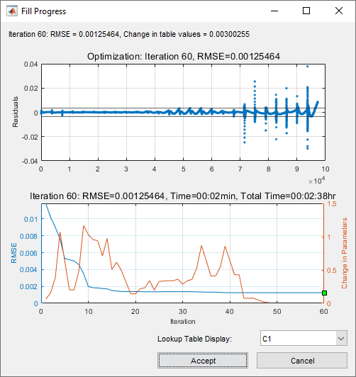
Before accepting an optimization, use the Fill Progress dialog box to review the results. Optimization runs can take a long time, possibly overnight. Click:
- Accept to use the lookup table values associated with the best solution found to date.
- Click Cancel if you want to discard the optimization run (for example, if the optimization is unstable). The table values are not changed. If necessary, you can Restart Optimization.
If CAGE displays a warning message about breakpoints, inspect the lookup tables and adjust the breakpoints. The warning message indicates that the lookup table has a mask that covers less than half the rows or columns.

Restart Optimization

You can restart the optimization by stopping and restarting the optimization. If you restart the optimization, CAGE initializes at the final values from the current lookup table. Consider:

Using optimization weights from a previous optimization.
Changing the learning rate if the previous run was unstable or if there was not much improvement.
Adjusting the smoothing factor to increase or decrease the table smoothness.
Adjusting the user-defined or time-based weights to put more emphasis on reducing high errors for specific data files.
Switching from Chebyshev to direct table fill when the fill starts to converge to realistic values.

Analyze Results

Use CAGE to analyze the feature fill results.

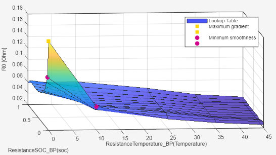
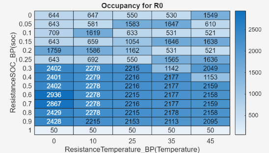
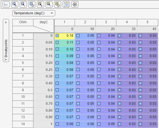
In the Fill Results section of the Feature Filling view, you can choose from these plot types to view the lookup table results:

Surface — View the lookup table surface.
Occupancy — View how much data is used for each lookup table cell.
Editor — Manually edit lookup table values. The extrapolation mask highlights table cells that the data uses. CAGE determines cells that the data uses by examining the derivatives of the feature with respect to table cells for columns containing nonzero entries.

Note
Selecting this option is an alternative to navigating to the Lookup Tables view to edit lookup table values.

On the Feature Filling pane, the Validation tab enables you to:

View the RMSE for each data file.
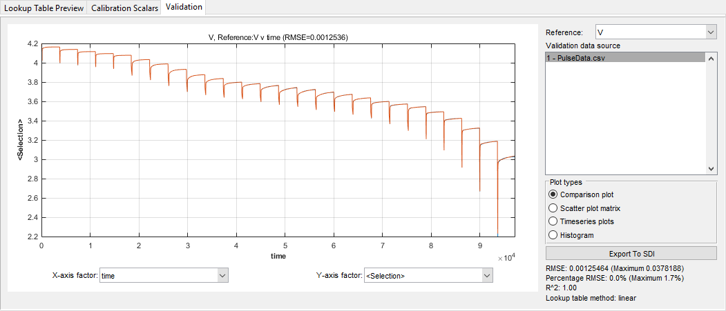
View the full-time trace of the optimization for a data file. Use the Validation data source to select a data file. Loading the full-time trace can take a long time for large data files.

Export Calibration

In CAGE, select File > Export > Calibration. You can export the tables in calibration formats, including INCA CSV file, INCA DCM file, and Simple CSV file.