Use Reject Inference Techniques with Credit Scorecards

This example demonstrates the hard-cutoff and fuzzy augmentation approaches to reject inference.

Reject inference is a method for improving the quality of a credit scorecard by incorporating data from rejected loan applications. Bias can result if a credit scorecard model is built only on accepts and does not account for applications rejected because of past denials for credit or unknown nondefault status. By using the reject inference method, you can infer the performance of rejects and include them in your credit scorecard model to remedy this bias.

To develop a credit scorecard, you must identify each borrower as either "good" or "bad". For rejected applications, information to identify borrowers as "good" or "bad" is not available. You cannot tell for sure to which group a borrower would have belonged had they been granted a loan. The reject inference method allows you to infer whether a borrower would likely be "good" or "bad" enabling you to incorporate the rejected application data into the data set that you use to build a credit scorecard.

As the diagram shows, reject inference requires that you determine the threshold (cutoff point) below which rejects are considered as "bad." This example demonstrates the hard-cutoff and the fuzzy augmentation approaches to calculate this threshold.

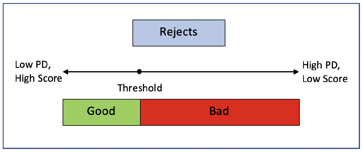
The following diagram shows the typical process for building a scorecard model. The red box represents the reject inference process, where the performance of the previously rejected applications is estimated and then used to re-train the credit scorecard model.

The workflow for the reject inference process is:

Build a logistic regression model based on the accepts.
Infer the class of rejects using one of the reject inference techniques.
Combine the accepts and rejects into a single data set.
Create a new scorecard, bin the expanded data set, and build a new logistic model.
Validate the final model.

There are two types of reject inference:

Simple assignment does not use a reject inference process and either ignores rejects or assigns all rejects to the "bad" class.
Augmentation uses a reject inference process to handle rejects based on a scoring model by combining the original data set with the rejects data.

This example focuses on augmentation techniques. The most popular techniques for augmentation are:

Simple augmentation — Using a cutoff value, this method assigns rejects with scores below and above the value to the "bad" or "good" class, respectively. The cutoff value must reflect that the rate of bads in the rejects is higher than in the accepted population. After the class ("good" or "bad") is assigned to the rejects, the entire population of accepts and rejects are fitted in the credit scorecard model and then scored. This approach is also called the hard-cutoff technique.
Fuzzy augmentation — This method scores the rejects by using a credit scorecard model based on the accepts. These rejects are duplicated into two observations, where each is assigned a probability of being "good" or "bad," and then aggregated to the accepts. A new credit scorecard model is then estimated on the new data set.

In this example, the following workflows are presented:

Both of these approaches use the binning rules preserved from the original scorecard and apply them to the new scorecard that is based on the combined data set.

Note: The data sets in this example are technically through-the-door (TTD) observations. That is, accepts and rejects are lumped together and differentiated based on their accept or reject decision. A rejects data set is then created from the TTD observations.

Hard-Cutoff Technique Workflow

The hard-cutoff technique uses a predefined cutoff value and assigns rejects below the cutoff as "bad" and above the cutoff as "good." The cutoff value must reflect that the rate of "bads" in the rejects is higher than in the accepts. After each reject is assigned a class ("good" or "bad"), the entire population of accepts and rejects is fitted in a credit scorecard model, and then that model is scored and validated. This approach is also called the simple augmentation technique. The main challenge in this approach is choosing the cutoff value.

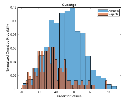
First, visualize the data for accepts and rejects for a selected predictor.

% Load the data
load CreditCardData.mat 
load RejectsCreditCardData.mat

Predictor = "CustAge";
figure;
h1 = histogram(data.(Predictor));
hold on
h2 = histogram(Rejects.(Predictor));
h1.Normalization = 'probability';
h2.Normalization = 'probability';
title(Predictor)
xlabel('Predictor Values')
ylabel('Normalized Count by Probability')
hold off
legend({'Accepts','Rejects'},'Location','best');

Figure contains an axes object. The axes object with title CustAge, xlabel Predictor Values, ylabel Normalized Count by Probability contains 2 objects of type histogram. These objects represent Accepts, Rejects.

Create a `creditscorecard` Object for the Accepts and Score the Data

Use creditscorecard to create a creditscorecard object that you can use to bin, fit, and then score the accepts.

scHC = creditscorecard(data,'IDVar','CustID');
scHC = autobinning(scHC);
scHC = fitmodel(scHC);

1. Adding CustIncome, Deviance = 1490.8527, Chi2Stat = 32.588614, PValue = 1.1387992e-08
2. Adding TmWBank, Deviance = 1467.1415, Chi2Stat = 23.711203, PValue = 1.1192909e-06
3. Adding AMBalance, Deviance = 1455.5715, Chi2Stat = 11.569967, PValue = 0.00067025601
4. Adding EmpStatus, Deviance = 1447.3451, Chi2Stat = 8.2264038, PValue = 0.0041285257
5. Adding CustAge, Deviance = 1441.994, Chi2Stat = 5.3511754, PValue = 0.020708306
6. Adding ResStatus, Deviance = 1437.8756, Chi2Stat = 4.118404, PValue = 0.042419078
7. Adding OtherCC, Deviance = 1433.707, Chi2Stat = 4.1686018, PValue = 0.041179769

Generalized linear regression model:
    logit(status) ~ 1 + CustAge + ResStatus + EmpStatus + CustIncome + TmWBank + OtherCC + AMBalance
    Distribution = Binomial

Estimated Coefficients:
                   Estimate       SE       tStat       pValue  
                   ________    ________    ______    __________

    (Intercept)    0.70239     0.064001    10.975    5.0538e-28
    CustAge        0.60833      0.24932      2.44      0.014687
    ResStatus        1.377      0.65272    2.1097      0.034888
    EmpStatus      0.88565        0.293    3.0227     0.0025055
    CustIncome     0.70164      0.21844    3.2121     0.0013179
    TmWBank         1.1074      0.23271    4.7589    1.9464e-06
    OtherCC         1.0883      0.52912    2.0569      0.039696
    AMBalance        1.045      0.32214    3.2439     0.0011792


1200 observations, 1192 error degrees of freedom
Dispersion: 1
Chi^2-statistic vs. constant model: 89.7, p-value = 1.4e-16

ScoreRange = [300 850];
scHC = formatpoints(scHC,'WorstAndBestScores',ScoreRange);
ScoresAccepts = score(scHC);

Choose a Bad Rate and Score the Rejects

A reject is "good" or "bad" based on the specified bad rate (BR) value. In general, the credit scoring industry assumes that rejects have a BR of 75%. This is a subjective evaluation that is usually based on an unknown value. In this example, you can adjust the value of BR.

The CreditCardData.mat input data has 'status' as response. Assume that GoodLabel (which means a nondefault) is the class that has a higher count in the response. In this example, GoodLabel is 0, which means that default only happens when the response is equal to 1.

% Define the BR
BR = 0.75;

% Sort rejects by ascending CustID order
N = height(Rejects);
Rejects = sortrows(Rejects);
ScoresRejects = score(scHC,Rejects);

% Find the lowest quantile based on the BR and set the corresponding observations to bad
BadLabel   = setdiff(unique(scHC.Data.(scHC.ResponseVar)),scHC.GoodLabel);
ScoreThres = quantile(ScoresRejects,BR);
ResponseRejects = zeros(N,1);
ResponseRejects(ScoresRejects < ScoreThres)  = BadLabel;
ResponseRejects(ScoresRejects >= ScoreThres) = scHC.GoodLabel;

% Create the rejects table
RejectsTable    = [Rejects table(ResponseRejects,'VariableNames',{scHC.ResponseVar})];

Combine Accepts and Rejects Into a New Data Set, Score, and Validate

To draw a more accurate comparison between the accepts and the combined data set, use the same binning rules from the initial accepts credit scorecard and copy them to the creditscorecard object built on the combined dataset. This ensures that the binning assignment does not affect the later comparison of the two credit scorecard models. Also, you can visualize how the rejects are spread out in the data range of each predictor.

% Create the final combined scorecard
CombinedData = [data(:,2:end);RejectsTable(:,2:end)];
scNewHC = creditscorecard(CombinedData,'GoodLabel',0);

% Bin using the same binning rules as the base scorecard
Predictors = scHC.PredictorVars;
Edges = struct();
for i = 1 : length(Predictors)
    Pred = Predictors{i};
    [bi,cp] = bininfo(scHC,Pred);
    if ismember(Pred,scHC.NumericPredictors)
        scNewHC = modifybins(scNewHC,Pred,'CutPoints',cp);
    else
        scNewHC = modifybins(scNewHC,Pred,'CatGrouping',cp);
    end
    Edges.(Pred) = bi.Bin(1:end-1);
end

% Visualize the rejects distribution in each bin
bd1 = bindata(scHC,data);
bd2 = bindata(scHC,CombinedData);
Predictor = "CustAge";
figure;
bar(categorical(Edges.(Predictor)),histcounts(bd1.(Predictor)))
hold on
bar(categorical(Edges.(Predictor)),histcounts(bd2.(Predictor)),'FaceAlpha',0.25)
hold off
xlabel('Bins')
ylabel('Counts')
legend({'Accepts Only','Combined'},'Location','best')

Figure contains an axes object. The axes object with xlabel Bins, ylabel Counts contains 2 objects of type bar. These objects represent Accepts Only, Combined.

Compare the initial creditscorecard object (scHC) to the new creditscorecard object (scNewHC) for the distribution of "goods" and "bads" for the selected predictor.

plotbins(scHC,Predictor);

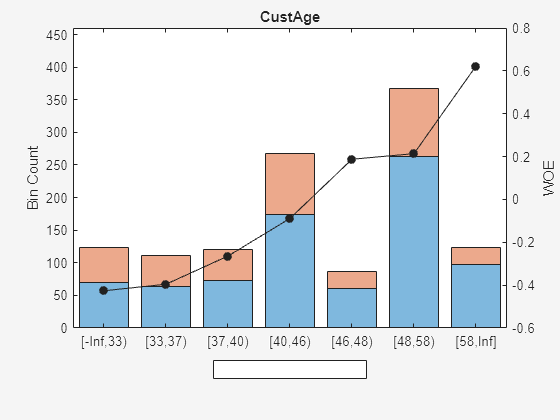
Figure contains an axes object. The axes object with title CustAge, ylabel WOE contains 3 objects of type bar, line. These objects represent Good, Bad.

plotbins(scNewHC,Predictor);

Figure contains an axes object. The axes object with title CustAge, ylabel WOE contains 3 objects of type bar, line. These objects represent Good, Bad.

Fit a logistic regression model for the creditscorecard object scNewHC and then score scNewHC.

scNewHC = fitmodel(scNewHC);

1. Adding CustIncome, Deviance = 1693.9882, Chi2Stat = 114.39516, PValue = 1.0676416e-26
2. Adding TmWBank, Deviance = 1650.6615, Chi2Stat = 43.326628, PValue = 4.6323638e-11
3. Adding AMBalance, Deviance = 1623.0668, Chi2Stat = 27.594773, PValue = 1.4958244e-07
4. Adding EmpStatus, Deviance = 1603.603, Chi2Stat = 19.463733, PValue = 1.0252802e-05
5. Adding CustAge, Deviance = 1592.3467, Chi2Stat = 11.256272, PValue = 0.00079354409
6. Adding ResStatus, Deviance = 1582.0086, Chi2Stat = 10.338134, PValue = 0.0013030966
7. Adding OtherCC, Deviance = 1572.1, Chi2Stat = 9.9086387, PValue = 0.0016450476

Generalized linear regression model:
    logit(status) ~ 1 + CustAge + ResStatus + EmpStatus + CustIncome + TmWBank + OtherCC + AMBalance
    Distribution = Binomial

Estimated Coefficients:
                   Estimate       SE       tStat       pValue  
                   ________    ________    ______    __________

    (Intercept)    0.48115     0.061301     7.849    4.1925e-15
    CustAge        0.50857      0.14449    3.5197    0.00043207
    ResStatus        1.151      0.34773    3.3101    0.00093262
    EmpStatus      0.78527      0.17826    4.4051    1.0572e-05
    CustIncome     0.68743      0.12372    5.5563    2.7555e-08
    TmWBank         1.0001      0.16731    5.9779    2.2607e-09
    OtherCC        0.97659      0.30956    3.1548     0.0016062
    AMBalance      0.91563      0.19073    4.8006    1.5819e-06


1361 observations, 1353 error degrees of freedom
Dispersion: 1
Chi^2-statistic vs. constant model: 236, p-value = 2.29e-47

scNewHC  = formatpoints(scNewHC,'WorstAndBestScores',ScoreRange);
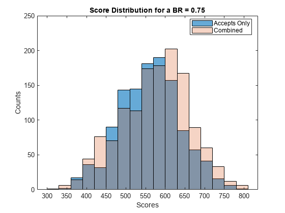
Scores = score(scNewHC);

% Visualize the score distribution
histogram(ScoresAccepts)

Warning: Error updating Legend.

 Property BaselineB_IS not found in class matlab.graphics.axis.PlotTarget, or is not present in all elements of the array of class matlab.graphics.axis.PlotTarget.

Warning: Error updating Legend.

 Property BaselineB_IS not found in class matlab.graphics.axis.PlotTarget, or is not present in all elements of the array of class matlab.graphics.axis.PlotTarget.

hold on
histogram(Scores,'FaceAlpha',0.25)
hold off
ylabel('Counts')
xlabel('Scores')
title(sprintf('Score Distribution for a BR = %.2f',BR))
legend({'Accepts Only','Combined'},'Location','best')

Figure contains an axes object. The axes object with title Score Distribution for a BR = 0.75, xlabel Scores, ylabel Counts contains 2 objects of type histogram. These objects represent Accepts Only, Combined.

Validate the Model on the Combined Data Set

Before validation, you must adjust the data set. To adjust the data set, you can either:

Validate the accepts for both scorecards
Validate the combined data set for both scorecards

% Get statistics for the accepts
StatsA1 = validatemodel(scHC);

Warning: Error updating Legend.

 Property BaselineB_IS not found in class matlab.graphics.axis.PlotTarget, or is not present in all elements of the array of class matlab.graphics.axis.PlotTarget.

Warning: Error updating Legend.

 Property BaselineB_IS not found in class matlab.graphics.axis.PlotTarget, or is not present in all elements of the array of class matlab.graphics.axis.PlotTarget.

Warning: Error updating Legend.

 Property BaselineB_IS not found in class matlab.graphics.axis.PlotTarget, or is not present in all elements of the array of class matlab.graphics.axis.PlotTarget.

StatsA2 = validatemodel(scNewHC,data);

% Get the statistics for the combined data set
StatsC1 = validatemodel(scHC,CombinedData);
StatsC2 = validatemodel(scNewHC);

s1 = table(StatsA1.Value,StatsA2.Value,'VariableNames',{'BaseScorecard','CombinedScorecard'});
s2 = table(StatsC1.Value,StatsC2.Value,'VariableNames',{'BaseScorecard','CombinedScorecard'});
Stats = table(StatsA1.Measure,s1,s2,'VariableNames',{'Measure','Accepts','Combined'}); 
disp(Stats)

            Measure                          Accepts                               Combined             
                                BaseScorecard    CombinedScorecard    BaseScorecard    CombinedScorecard
    ________________________    __________________________________    __________________________________

    {'Accuracy Ratio'      }       0.32258            0.31695            0.47022            0.46565     
    {'Area under ROC curve'}       0.66129            0.65848            0.73511            0.73282     
    {'KS statistic'        }        0.2246            0.22946            0.34528            0.33681     
    {'KS score'            }        550.72             576.57             512.44             542.85

Fuzzy Augmentation Technique Workflow

The Fuzzy augmentation technique starts by building a scorecard using the accepts only and then this scorecard model is used to score the rejects. Unlike the hard-cutoff technique, the fuzzy augmentation approach does not assign "good" or "bad" classes. Rather, each reject is duplicated into two observations and assigned a weighted "good" or "bad" value, based on a probability of being "good" or "bad." The weighted rejects are then added to the accepts data set and the combined data set is used to create a scorecard that is then fit and validated.

First, visualize the data for accepts and rejects for a selected predictor.

% Load the data
load CreditCardData.mat
load RejectsCreditCardData.mat

Predictor = "CustAge";
figure;
h1 = histogram(data.(Predictor));
hold on
h2 = histogram(Rejects.(Predictor));
h1.Normalization = 'probability';
h2.Normalization = 'probability';
title(Predictor)
xlabel('Predictor values')
ylabel('Normalized Count by Probability')
hold off
legend({'Accepts','Rejects'},'Location','best');

Figure contains an axes object. The axes object with title CustAge, xlabel Predictor values, ylabel Normalized Count by Probability contains 2 objects of type histogram. These objects represent Accepts, Rejects.

Create a `creditscorecard` Object for the Accepts and Score the Data

Use creditscorecard to create a creditscorecard object for the accepts, which you can bin, fit, and then score.

scFA = creditscorecard(data,'IDVar','CustID');
scFA = autobinning(scFA);
scFA = fitmodel(scFA);

1. Adding CustIncome, Deviance = 1490.8527, Chi2Stat = 32.588614, PValue = 1.1387992e-08
2. Adding TmWBank, Deviance = 1467.1415, Chi2Stat = 23.711203, PValue = 1.1192909e-06
3. Adding AMBalance, Deviance = 1455.5715, Chi2Stat = 11.569967, PValue = 0.00067025601
4. Adding EmpStatus, Deviance = 1447.3451, Chi2Stat = 8.2264038, PValue = 0.0041285257
5. Adding CustAge, Deviance = 1441.994, Chi2Stat = 5.3511754, PValue = 0.020708306
6. Adding ResStatus, Deviance = 1437.8756, Chi2Stat = 4.118404, PValue = 0.042419078
7. Adding OtherCC, Deviance = 1433.707, Chi2Stat = 4.1686018, PValue = 0.041179769

Generalized linear regression model:
    logit(status) ~ 1 + CustAge + ResStatus + EmpStatus + CustIncome + TmWBank + OtherCC + AMBalance
    Distribution = Binomial

Estimated Coefficients:
                   Estimate       SE       tStat       pValue  
                   ________    ________    ______    __________

    (Intercept)    0.70239     0.064001    10.975    5.0538e-28
    CustAge        0.60833      0.24932      2.44      0.014687
    ResStatus        1.377      0.65272    2.1097      0.034888
    EmpStatus      0.88565        0.293    3.0227     0.0025055
    CustIncome     0.70164      0.21844    3.2121     0.0013179
    TmWBank         1.1074      0.23271    4.7589    1.9464e-06
    OtherCC         1.0883      0.52912    2.0569      0.039696
    AMBalance        1.045      0.32214    3.2439     0.0011792


1200 observations, 1192 error degrees of freedom
Dispersion: 1
Chi^2-statistic vs. constant model: 89.7, p-value = 1.4e-16

ScoreRange = [300 850];
scFA = formatpoints(scFA,'WorstAndBestScores',ScoreRange);
ScoresAccepts = score(scFA);

Score the Rejects and Create the Combined Data Set

% Load the rejects dataset and score the observations
load RejectsCreditCardData.mat

ScoresRejects = score(scFA,Rejects);

% Compute the probabilities of default and use as weights
pdRejects = probdefault(scFA,Rejects);

% Assign bad status to pd (probability of default) and good status to 1-pd weights
BadLabel = setdiff(unique(scFA.Data.(scFA.ResponseVar)),scFA.GoodLabel);
Weights  = zeros(2*length(pdRejects),1);
Response = zeros(2*length(pdRejects),1);
Weights(1:2:end)  = pdRejects;
Response(1:2:end) = BadLabel;
Weights(2:2:end)  = 1-pdRejects;
Response(2:2:end) = scFA.GoodLabel;

% Rearrange the response so that each two rows correspond to the same
% observation from rejects
RejectsTable = repelem(Rejects(:,2:end),2,1);
RejectsTable = addvars(RejectsTable,Weights,Response,'NewVariableNames',...
    {'Weights',scFA.ResponseVar});

% Combine accepts and rejects
AcceptsData = addvars(data,ones(height(data),1),'Before',scFA.ResponseVar,...
    'NewVariableNames','Weights');
CombinedData = [AcceptsData(:,2:end);RejectsTable];

Combine Accepts and Rejects into a New Data Set, Score, and Validate

To draw a more accurate comparison between the accepts and the combined data set, use the same binning rules from the initial accepts credit scorecard and copy them to the creditscorecard object built on the combined dataset. This ensures that the binning assignments does not affect the later comparison of the two credit scorecard models. Also, you can visualize how the rejects are spread out in the data range of each predictor.

scNewFA = creditscorecard(CombinedData,'GoodLabel',0,'WeightsVar','Weights');

% Bin using the same binning rules as the base scorecard
Predictors = scFA.PredictorVars;
Edges = struct();
for i = 1 : length(Predictors)
    Pred = Predictors{i};
    [bi,cp] = bininfo(scFA,Pred);
    if ismember(Pred,scFA.NumericPredictors)
        scNewFA = modifybins(scNewFA,Pred,'CutPoints',cp);
    else
        scNewFA = modifybins(scNewFA,Pred,'CatGrouping',cp);
    end
    Edges.(Pred) = bi.Bin(1:end-1);
end

% Visualize the rejects distribution in each bin
bd1 = bindata(scFA,data);
bd2 = bindata(scFA,CombinedData);
Predictor = "CustAge";
figure;
bar(categorical(Edges.(Predictor)),histcounts(bd1.(Predictor)))
hold on
bar(categorical(Edges.(Predictor)),histcounts(bd2.(Predictor)),'FaceAlpha',0.25)
hold off
xlabel('Bins')
ylabel('Counts')
legend({'Accepts Only','Combined'},'Location','best')

Figure contains an axes object. The axes object with xlabel Bins, ylabel Counts contains 2 objects of type bar. These objects represent Accepts Only, Combined.

Compare the initial creditscorecard object (scFA) to the new creditscorecard object (scNewFA) for the distribution of "goods" and "bads" for the selected predictor.

plotbins(scFA,Predictor);

Figure contains an axes object. The axes object with title CustAge, ylabel WOE contains 3 objects of type bar, line. These objects represent Good, Bad.

plotbins(scNewFA,Predictor);

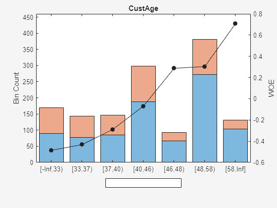
Figure contains an axes object. The axes object with title CustAge, ylabel WOE contains 3 objects of type bar, line. These objects represent Good, Bad.

Fit a logistic regression model for the creditscorecard object scNewFA and then score scNewFA.

scNewFA = fitmodel(scNewFA);

1. Adding CustIncome, Deviance = 1711.3102, Chi2Stat = 54.160619, PValue = 1.8475277e-13
2. Adding TmWBank, Deviance = 1682.5353, Chi2Stat = 28.774866, PValue = 8.1299351e-08
3. Adding AMBalance, Deviance = 1668.2956, Chi2Stat = 14.239727, PValue = 0.00016093686
4. Adding EmpStatus, Deviance = 1658.2944, Chi2Stat = 10.001236, PValue = 0.001564352
5. Adding CustAge, Deviance = 1652.3976, Chi2Stat = 5.8967925, PValue = 0.015168483
6. Adding OtherCC, Deviance = 1647.7632, Chi2Stat = 4.6344022, PValue = 0.031337059
7. Adding ResStatus, Deviance = 1642.8332, Chi2Stat = 4.9299914, PValue = 0.026394448

Generalized linear regression model:
    logit(status) ~ 1 + CustAge + ResStatus + EmpStatus + CustIncome + TmWBank + OtherCC + AMBalance
    Distribution = Binomial

Estimated Coefficients:
                   Estimate       SE       tStat       pValue  
                   ________    ________    ______    __________

    (Intercept)    0.60838     0.059654    10.198    2.0142e-24
    CustAge        0.50755      0.20092    2.5262      0.011532
    ResStatus        1.082      0.48919    2.2119      0.026971
    EmpStatus      0.74776      0.23526    3.1784     0.0014809
    CustIncome      0.6372      0.17519    3.6371    0.00027567
    TmWBank        0.96561      0.19664    4.9106    9.0815e-07
    OtherCC        0.90699      0.40476    2.2408      0.025039
    AMBalance      0.87642      0.25404    3.4499    0.00056077


1522 observations, 1514 error degrees of freedom
Dispersion: 1
Chi^2-statistic vs. constant model: 123, p-value = 2.16e-23

scNewFA  = formatpoints(scNewFA,'WorstAndBestScores',ScoreRange);
Scores = score(scNewFA);
pd = probdefault(scNewFA);

% Visualize the score distribution
histogram(ScoresAccepts)

Warning: Error updating Legend.

 Property BaselineB_IS not found in class matlab.graphics.axis.PlotTarget, or is not present in all elements of the array of class matlab.graphics.axis.PlotTarget.

Warning: Error updating Legend.

 Property BaselineB_IS not found in class matlab.graphics.axis.PlotTarget, or is not present in all elements of the array of class matlab.graphics.axis.PlotTarget.

hold on
histogram(Scores,'FaceAlpha',0.25)
hold off
ylabel('Counts')
xlabel('Scores')
title('Score Distribution Using Fuzzy Augmentation')
legend({'Accepts Only','Combined'},'Location','best')

Figure contains an axes object. The axes object with title Score Distribution Using Fuzzy Augmentation, xlabel Scores, ylabel Counts contains 2 objects of type histogram. These objects represent Accepts Only, Combined.

Validate the Model on the Combined Data Set

Before validation, you must adjust the data set. To adjust the data set, you can either:

Validate the accepts for both scorecards
Validate the combined data set for both scorecards

% Get statistics for the accepts
data.Weights = ones(height(data),1);

Warning: Error updating Legend.

 Property BaselineB_IS not found in class matlab.graphics.axis.PlotTarget, or is not present in all elements of the array of class matlab.graphics.axis.PlotTarget.

Warning: Error updating Legend.

 Property BaselineB_IS not found in class matlab.graphics.axis.PlotTarget, or is not present in all elements of the array of class matlab.graphics.axis.PlotTarget.

Warning: Error updating Legend.

 Property BaselineB_IS not found in class matlab.graphics.axis.PlotTarget, or is not present in all elements of the array of class matlab.graphics.axis.PlotTarget.

Warning: Error updating Legend.

 Property BaselineB_IS not found in class matlab.graphics.axis.PlotTarget, or is not present in all elements of the array of class matlab.graphics.axis.PlotTarget.

StatsA1 = validatemodel(scFA);
StatsA2 = validatemodel(scNewFA,data);
% Get the statistics for the combined data set
StatsC1 = validatemodel(scFA,CombinedData);
StatsC2 = validatemodel(scNewFA);

s1 = table(StatsA1.Value,StatsA2.Value,'VariableNames',{'BaseScorecard','CombinedScorecard'});
s2 = table(StatsC1.Value,StatsC2.Value,'VariableNames',{'BaseScorecard','CombinedScorecard'});
Stats = table(StatsA1.Measure,s1,s2,'VariableNames',{'Measure','Accepts','Combined'}); 
disp(Stats)

            Measure                          Accepts                               Combined             
                                BaseScorecard    CombinedScorecard    BaseScorecard    CombinedScorecard
    ________________________    __________________________________    __________________________________

    {'Accuracy Ratio'      }       0.32258            0.32088            0.29419            0.35143     
    {'Area under ROC curve'}       0.66129            0.66044            0.64709            0.67571     
    {'KS statistic'        }        0.2246            0.22799            0.22596            0.25629     
    {'KS score'            }        550.72             554.84             512.44             520.99

Summary

This example demonstrates how to use a reject inference process within the framework of the credit scorecard workflow. The Hard-Cutoff and the Fuzzy Augmentation techniques show how you can bin the data, fit a model, integrate the rejects with the accepts into a new credit scorecard model, and then validate the new credit scorecard model.

There is no clear-cut conclusion for which of these reject inference approaches is the best. This example is intended to illustrate how to use the features of creditscorecard to implement two different reject inference approaches.

References

Baesesn, B., D. Rösch, and H. Scheule. Credit Risk Analytics: Measurement Techniques, Applications and Examples in SAS. Wiley and SAS Business Series, 2016.
Refaat, M. Credit Risk Scorecards: Development and Implementation Using SAS. lulu.com, 2011.

Related Examples

More About

External Websites

Credit Scorecard Modeling Using the Binning Explorer App (6 min 17 sec)

Use Reject Inference Techniques with Credit Scorecards

Hard-Cutoff Technique Workflow

Create a creditscorecard Object for the Accepts and Score the Data

Choose a Bad Rate and Score the Rejects

Combine Accepts and Rejects Into a New Data Set, Score, and Validate

Validate the Model on the Combined Data Set

Fuzzy Augmentation Technique Workflow

Create a creditscorecard Object for the Accepts and Score the Data

Score the Rejects and Create the Combined Data Set

Combine Accepts and Rejects into a New Data Set, Score, and Validate

Validate the Model on the Combined Data Set

Summary

References

See Also

Related Examples

More About

External Websites

Create a `creditscorecard` Object for the Accepts and Score the Data

Create a `creditscorecard` Object for the Accepts and Score the Data