Stress Testing of Consumer Credit Default Probabilities Using Panel Data

Open Live Script

This example shows how to work with consumer (retail) credit panel data to visualize observed default rates at different levels. It also shows how to fit a model to predict probabilities of default (PD) and lifetime PD values, and perform a stress-testing analysis.

The panel data set of consumer loans enables you to identify default rate patterns for loans of different ages, or years on books. You can use information about a score group to distinguish default rates for different score levels. In addition, you can use macroeconomic information to assess how the state of the economy affects consumer loan default rates.

A standard logistic regression model, a type of generalized linear model, is fitted to the retail credit panel data with and without macroeconomic predictors, using fitLifetimePDModel from Risk Management Toolbox™. Although the same model can be fitted using the fitglm function from Statistics and Machine Learning Toolbox™, the lifetime probability of default (PD) version of the model is designed for credit applications, and supports lifetime PD prediction and model validation tools, including the discrimination and accuracy plots shown in this example. The example also describes how to fit a more advanced model to account for panel data effects, a generalized linear mixed effects model. However, the panel effects are negligible for the data set in this example and the standard logistic model is preferred for efficiency.

The logistic regression model predicts probabilities of default for all score levels, years on books, and macroeconomic variable scenarios. There is a brief discussion on how to predict lifetime PD values, with pointers to additional functionality. The example shows model discrimination and model accuracy tools to validate and compare models. In the last section of this example, the logistic model is used for a stress-testing analysis, the model predicts probabilities of default for a given baseline, as well as default probabilities for adverse and severely adverse macroeconomic scenarios.

For additional information, refer to Overview of Lifetime Probability of Default Models. See also the example Modeling Probabilities of Default with Cox Proportional Hazards, which follows the same workflow but uses Cox regression instead of logistic regression and also has information on the computation of lifetime PD and lifetime Expected Credit Loss (ECL).

Panel Data Description

The main data set (data) contains the following variables:

ID: Loan identifier.
ScoreGroup: Credit score at the beginning of the loan, discretized into three groups: High Risk, Medium Risk, and Low Risk.
YOB: Years on books.
Default: Default indicator. This is the response variable.
Year: Calendar year.

There is also a small data set (dataMacro) with macroeconomic data for the corresponding calendar years:

Year: Calendar year.
GDP: Gross domestic product growth (year over year).
Market: Market return (year over year).

The variables YOB, Year, GDP, and Market are observed at the end of the corresponding calendar year. The score group is a discretization of the original credit score when the loan started. A value of 1 for Default means that the loan defaulted in the corresponding calendar year.

There is also a third data set (dataMacroStress) with baseline, adverse, and severely adverse scenarios for the macroeconomic variables. This table is used for the stress-testing analysis.

This example uses simulated data, but the same approach has been successfully applied to real data sets.

Load the Panel Data

Load the data and view the first 10 and last 10 rows of the table. The panel data is stacked, in the sense that observations for the same ID are stored in contiguous rows, creating a tall, thin table. The panel is unbalanced, because not all IDs have the same number of observations.

load RetailCreditPanelData.mat

fprintf('\nFirst ten rows:\n')

First ten rows:

disp(data(1:10,:))

    ID    ScoreGroup     YOB    Default    Year
    __    ___________    ___    _______    ____

    1     Low Risk        1        0       1997
    1     Low Risk        2        0       1998
    1     Low Risk        3        0       1999
    1     Low Risk        4        0       2000
    1     Low Risk        5        0       2001
    1     Low Risk        6        0       2002
    1     Low Risk        7        0       2003
    1     Low Risk        8        0       2004
    2     Medium Risk     1        0       1997
    2     Medium Risk     2        0       1998

fprintf('Last ten rows:\n')

Last ten rows:

disp(data(end-9:end,:))

     ID      ScoreGroup     YOB    Default    Year
    _____    ___________    ___    _______    ____

    96819    High Risk       6        0       2003
    96819    High Risk       7        0       2004
    96820    Medium Risk     1        0       1997
    96820    Medium Risk     2        0       1998
    96820    Medium Risk     3        0       1999
    96820    Medium Risk     4        0       2000
    96820    Medium Risk     5        0       2001
    96820    Medium Risk     6        0       2002
    96820    Medium Risk     7        0       2003
    96820    Medium Risk     8        0       2004

nRows = height(data);
UniqueIDs = unique(data.ID);
nIDs = length(UniqueIDs);

fprintf('Total number of IDs: %d\n',nIDs)

Total number of IDs: 96820

fprintf('Total number of rows: %d\n',nRows)

Total number of rows: 646724

Default Rates by Score Groups and Years on Books

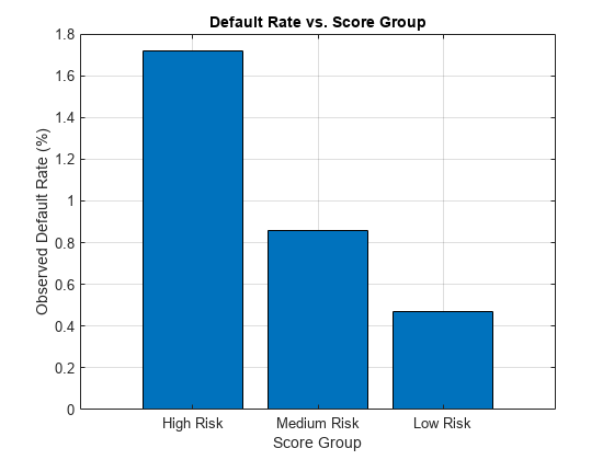
Use the credit score group as a grouping variable to compute the observed default rate for each score group. For this, use the groupsummary function to compute the mean of the Default variable, grouping by the ScoreGroup variable. Plot the results on a bar chart. As expected, the default rate goes down as the credit quality improves.

DefRateByScore = groupsummary(data,'ScoreGroup','mean','Default');
NumScoreGroups = height(DefRateByScore);

disp(DefRateByScore)

    ScoreGroup     GroupCount    mean_Default
    ___________    __________    ____________

    High Risk      2.0999e+05      0.017167  
    Medium Risk    2.1743e+05     0.0086006  
    Low Risk        2.193e+05     0.0046784

bar(DefRateByScore.ScoreGroup,DefRateByScore.mean_Default*100)
title('Default Rate vs. Score Group')
xlabel('Score Group')
ylabel('Observed Default Rate (%)')
grid on

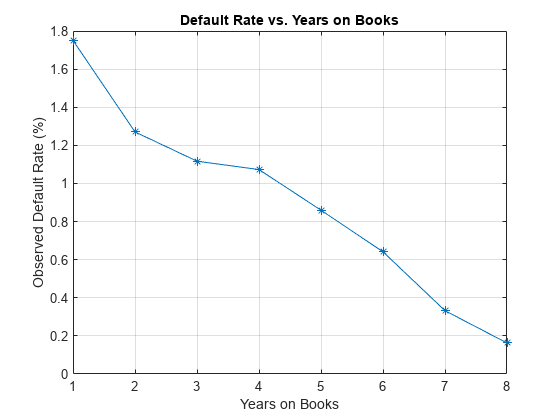
Figure contains an axes object. The axes object with title Default Rate vs. Score Group, xlabel Score Group, ylabel Observed Default Rate (%) contains an object of type bar.

Next, compute default rates grouping by years on books (represented by the YOB variable). The resulting rates are conditional one-year default rates. For example, the default rate for the third year on books is the proportion of loans defaulting in the third year, relative to the number of loans that are in the portfolio past the second year. In other words, the default rate for the third year is the number of rows with YOB = 3 and Default = 1, divided by the number of rows with YOB = 3.

Plot the results. There is a clear downward trend, with default rates going down as the number of years on books increases. Years three and four have similar default rates. However, it is unclear from this plot whether this is a characteristic of the loan product or an effect of the macroeconomic environment.

DefRateByYOB = groupsummary(data,'YOB','mean','Default');
NumYOB = height(DefRateByYOB);

disp(DefRateByYOB)

    YOB    GroupCount    mean_Default
    ___    __________    ____________

     1       96820         0.017507  
     2       94535         0.012704  
     3       92497         0.011168  
     4       91068         0.010728  
     5       89588        0.0085949  
     6       88570         0.006413  
     7       61689        0.0033231  
     8       31957        0.0016272

plot(double(DefRateByYOB.YOB),DefRateByYOB.mean_Default*100,'-*')
title('Default Rate vs. Years on Books')
xlabel('Years on Books')
ylabel('Observed Default Rate (%)')
grid on

Figure contains an axes object. The axes object with title Default Rate vs. Years on Books, xlabel Years on Books, ylabel Observed Default Rate (%) contains an object of type line.

Now, group both by the score group and number of years on books and then plot the results. The plot shows that all score groups behave similarly as time progresses, with a general downward trend. Years three and four are an exception to the downward trend: the rates flatten for the High Risk group, and go up in year three for the Low Risk group.

DefRateByScoreYOB = groupsummary(data,{'ScoreGroup','YOB'},'mean','Default');

% Display output table to show the way it is structured
% Display only the first 10 rows, for brevity
disp(DefRateByScoreYOB(1:10,:))

    ScoreGroup     YOB    GroupCount    mean_Default
    ___________    ___    __________    ____________

    High Risk       1       32601         0.029692  
    High Risk       2       31338         0.021252  
    High Risk       3       30138         0.018448  
    High Risk       4       29438         0.018276  
    High Risk       5       28661         0.014794  
    High Risk       6       28117         0.011168  
    High Risk       7       19606        0.0056615  
    High Risk       8       10094        0.0027739  
    Medium Risk     1       32373         0.014302  
    Medium Risk     2       31775         0.011676

DefRateByScoreYOB2 = reshape(DefRateByScoreYOB.mean_Default,...
   NumYOB,NumScoreGroups);

plot(DefRateByScoreYOB2*100,'-*')
title('Default Rate vs. Years on Books')
xlabel('Years on Books')
ylabel('Observed Default Rate (%)')
legend(categories(data.ScoreGroup))
grid on

Figure contains an axes object. The axes object with title Default Rate vs. Years on Books, xlabel Years on Books, ylabel Observed Default Rate (%) contains 3 objects of type line. These objects represent High Risk, Medium Risk, Low Risk.

Years on Books Versus Calendar Years

The data contains three cohorts, or vintages: loans started in 1997, 1998, and 1999. No loan in the panel data started after 1999.

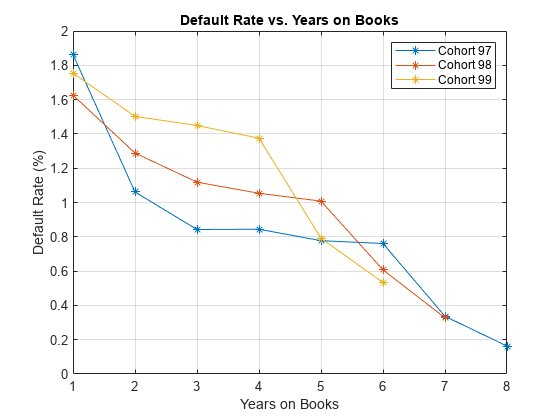
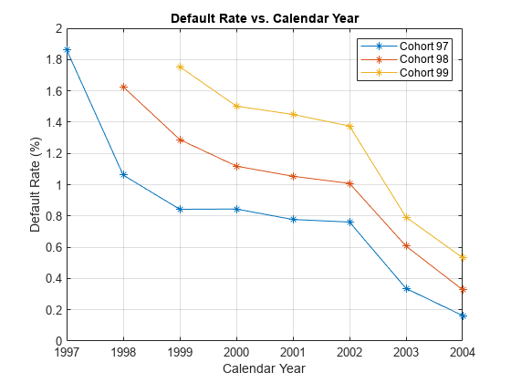
This section shows how to visualize the default rate for each cohort separately. The default rates for all cohorts are plotted, both against the number of years on books and against the calendar year. Patterns in the years on books suggest the loan product characteristics. Patterns in the calendar years suggest the influence of the macroeconomic environment.

From years two through four on books, the curves show different patterns for the three cohorts. When plotted against the calendar year, however, the three cohorts show similar behavior from 2000 through 2002. The curves flatten during that period.

% Get IDs of 1997, 1998, and 1999 cohorts
IDs1997 = data.ID(data.YOB==1&data.Year==1997);
IDs1998 = data.ID(data.YOB==1&data.Year==1998);
IDs1999 = data.ID(data.YOB==1&data.Year==1999);
% IDs2000AndUp is unused, it is only computed to show that this is empty,
% no loans started after 1999
IDs2000AndUp = data.ID(data.YOB==1&data.Year>1999);

% Get default rates for each cohort separately
ObsDefRate1997 = groupsummary(data(ismember(data.ID,IDs1997),:),...
    'YOB','mean','Default');

ObsDefRate1998 = groupsummary(data(ismember(data.ID,IDs1998),:),...
    'YOB','mean','Default');

ObsDefRate1999 = groupsummary(data(ismember(data.ID,IDs1999),:),...
    'YOB','mean','Default');

% Plot against the years on books
plot(ObsDefRate1997.YOB,ObsDefRate1997.mean_Default*100,'-*')
hold on
plot(ObsDefRate1998.YOB,ObsDefRate1998.mean_Default*100,'-*')
plot(ObsDefRate1999.YOB,ObsDefRate1999.mean_Default*100,'-*')
hold off
title('Default Rate vs. Years on Books')
xlabel('Years on Books')
ylabel('Default Rate (%)')
legend('Cohort 97','Cohort 98','Cohort 99')
grid on

Figure contains an axes object. The axes object with title Default Rate vs. Years on Books, xlabel Years on Books, ylabel Default Rate (%) contains 3 objects of type line. These objects represent Cohort 97, Cohort 98, Cohort 99.

% Plot against the calendar year
Year = unique(data.Year);

plot(Year,ObsDefRate1997.mean_Default*100,'-*')
hold on
plot(Year(2:end),ObsDefRate1998.mean_Default*100,'-*')
plot(Year(3:end),ObsDefRate1999.mean_Default*100,'-*')
hold off
title('Default Rate vs. Calendar Year')
xlabel('Calendar Year')
ylabel('Default Rate (%)')
legend('Cohort 97','Cohort 98','Cohort 99')
grid on

Figure contains an axes object. The axes object with title Default Rate vs. Calendar Year, xlabel Calendar Year, ylabel Default Rate (%) contains 3 objects of type line. These objects represent Cohort 97, Cohort 98, Cohort 99.

Model of Default Rates Using Score Group and Years on Books

After you visualize the data, you can build predictive models for the default rates.

Split the panel data into training and testing sets, defining these sets based on ID numbers.

NumTraining = floor(0.6*nIDs);

rng('default'); % for reproducibility
TrainIDInd = randsample(nIDs,NumTraining);
TrainDataInd = ismember(data.ID,UniqueIDs(TrainIDInd));
TestDataInd = ~TrainDataInd;

The first model uses only score group and number of years on books as predictors of the default rate p. The odds of defaulting are defined as p/(1-p). The logistic model relates the logarithm of the odds, or log odds, to the predictors as follows:

$\log (\frac{p}{1 - p}) = a_{H} + a_{M} 1_{M} + a_{L} 1_{L} + b_{Y O B} Y O B + ϵ$

1M is an indicator with a value 1 for Medium Risk loans and 0 otherwise, and similarly for 1L for Low Risk loans. This is a standard way of handling a categorical predictor such as ScoreGroup. There is effectively a different constant for each risk level: aH for High Risk, aH+aM for Medium Risk, and aH+aL for Low Risk.

ModelNoMacro = fitLifetimePDModel(data(TrainDataInd,:),'logistic',...
   'ModelID','No Macro','Description','Logistic model with YOB and score group, but no macro variables',...
   'IDVar','ID','LoanVars','ScoreGroup','AgeVar','YOB','ResponseVar','Default');
disp(ModelNoMacro.UnderlyingModel)

Compact generalized linear regression model:
    logit(Default) ~ 1 + ScoreGroup + YOB
    Distribution = Binomial

Estimated Coefficients:
                              Estimate       SE        tStat       pValue   
                              ________    ________    _______    ___________

    (Intercept)                -3.2453    0.033768    -96.106              0
    ScoreGroup_Medium Risk     -0.7058    0.037103    -19.023     1.1014e-80
    ScoreGroup_Low Risk        -1.2893    0.045635    -28.253    1.3076e-175
    YOB                       -0.22693    0.008437    -26.897    2.3578e-159


388018 observations, 388014 error degrees of freedom
Dispersion: 1
Chi^2-statistic vs. constant model: 1.83e+03, p-value = 0

For any row in the data, the value of p is not observed, only a 0 or 1 default indicator is observed. The calibration finds model coefficients, and the predicted values of p for individual rows can be recovered with the predict function.

The Intercept coefficient is the constant for the High Risk level (the aH term), and the ScoreGroup_Medium Risk and ScoreGroup_Low Risk coefficients are the adjustments for Medium Risk and Low Risk levels (the aM and aL terms).

The default probability p and the log odds (the left side of the model) move in the same direction when the predictors change. Therefore, because the adjustments for Medium Risk and Low Risk are negative, the default rates are lower for better risk levels, as expected. The coefficient for number of years on books is also negative, consistent with the overall downward trend for number of years on books observed in the data.

An alternative way to fit the model is using the fitglm function from Statistics and Machine Learning Toolbox™. The formula above is expressed as

Default ~ 1 + ScoreGroup + YOB

The 1 + ScoreGroup terms account for the baseline constant and the adjustments for risk level. Set the optional argument Distribution to binomial to indicate that a logistic model is desired (that is, a model with log odds on the left side), as follows:

ModelNoMacro = fitglm(data(TrainDataInd,:), 'Default ~ 1 + ScoreGroup + YOB','Distribution','binomial');

As mentioned in the introduction, the advantage of the lifetime PD version of the model fitted with fitLifetimePDModel is that it is designed for credit applications, and it can predict lifetime PD and supports model validation tools, including the discrimination and accuracy plots. For more information, see Overview of Lifetime Probability of Default Models.

To account for panel data effects, a more advanced model using mixed effects can be fitted using the fitglme function from Statistics and Machine Learning Toolbox™. Although this model is not fitted in this example, the code is very similar:

ModelNoMacro = fitglme(data(TrainDataInd,:),'Default ~ 1 + ScoreGroup + YOB + (1|ID)','Distribution','binomial');

The (1|ID) term in the formula adds a random effect to the model. This effect is a predictor whose values are not given in the data, but fitted together with the model coefficients. A random value is fit for each ID. This additional fitting requirement substantially increases the computational time to fit the model in this case, because of the very large number of IDs. For the panel data set in this example, the random term has a negligible effect. The variance of the random effects is very small and the model coefficients barely change when the random effect is introduced. The simpler logistic regression model is preferred, because it is faster to fit and to predict, and the default rates predicted with both models are essentially the same.

Predict the probability of default for training and testing data. The predict function predicts conditional PD values, row by row. We store the data to compare the predictions against the macro model in the next section.

data.PDNoMacro = zeros(height(data),1);

% Predict in-sample
data.PDNoMacro(TrainDataInd) = predict(ModelNoMacro,data(TrainDataInd,:));
% Predict out-of-sample
data.PDNoMacro(TestDataInd) = predict(ModelNoMacro,data(TestDataInd,:));

To make lifetime PD predictions, use the predictLifetime function. For lifetime predictions, projected values of the predictors are required for each ID value in the prediction data set. For example, predict the survival probability for the first two IDs in the dataset. See how the conditional PD (PDNoMacro column) and the lifetime PD (LifetimePD column) match for the first year of each ID. After that year, the lifetime PD increases because it is a cumulative probability. For more information, see predictLifetime. See also the Expected Credit Loss Computation example.

data1 = data(1:16,:);
data1.LifetimePD = predictLifetime(ModelNoMacro,data1);
disp(data1)

    ID    ScoreGroup     YOB    Default    Year    PDNoMacro    LifetimePD
    __    ___________    ___    _______    ____    _________    __________

    1     Low Risk        1        0       1997    0.0084797    0.0084797 
    1     Low Risk        2        0       1998    0.0067697     0.015192 
    1     Low Risk        3        0       1999    0.0054027     0.020513 
    1     Low Risk        4        0       2000    0.0043105     0.024735 
    1     Low Risk        5        0       2001    0.0034384     0.028088 
    1     Low Risk        6        0       2002    0.0027422     0.030753 
    1     Low Risk        7        0       2003    0.0021867     0.032873 
    1     Low Risk        8        0       2004    0.0017435     0.034559 
    2     Medium Risk     1        0       1997     0.015097     0.015097 
    2     Medium Risk     2        0       1998     0.012069     0.026984 
    2     Medium Risk     3        0       1999    0.0096422     0.036366 
    2     Medium Risk     4        0       2000    0.0076996     0.043785 
    2     Medium Risk     5        0       2001     0.006146     0.049662 
    2     Medium Risk     6        0       2002    0.0049043     0.054323 
    2     Medium Risk     7        0       2003    0.0039125     0.058023 
    2     Medium Risk     8        0       2004    0.0031207     0.060962

Visualize the in-sample (training) or out-of-sample (test) fit using modelCalibrationPlot. It requires a grouping variable to compute default rates and average predicted PD values for each group. Use the years on books as grouping variable here.

DataSetChoice = "Test";
if DataSetChoice=="Training"
   Ind = TrainDataInd;
else
   Ind = TestDataInd;
end
modelCalibrationPlot(ModelNoMacro,data(Ind,:),'YOB','DataID',DataSetChoice)

Figure contains an axes object. The axes object with title Scatter Grouped by YOB Test No Macro, RMSE = 0.001349, xlabel YOB, ylabel PD contains 2 objects of type line. One or more of the lines displays its values using only markers These objects represent Observed, No Macro.

The score group can be input as a second grouping variable to visualize the fit by score groups.

modelCalibrationPlot(ModelNoMacro,data(Ind,:),{'YOB' 'ScoreGroup'},'DataID',DataSetChoice)

Figure contains an axes object. The axes object with title Scatter Grouped by YOB and ScoreGroup Test No Macro, RMSE = 0.0016366, xlabel YOB, ylabel PD contains 6 objects of type line. One or more of the lines displays its values using only markers These objects represent High Risk, Observed, Medium Risk, Observed, Low Risk, Observed, High Risk, No Macro, Medium Risk, No Macro, Low Risk, No Macro.

Lifetime PD models also support validation tools for model discrimination. In particular, the modelDiscriminationPlot function creates the receiver operating characteristic (ROC) curve plot. Here a separate ROC curve is requested for each score group. For more information, see modelDiscriminationPlot.

modelDiscriminationPlot(ModelNoMacro,data(Ind,:),'SegmentBy','ScoreGroup','DataID',DataSetChoice)

Figure contains an axes object. The axes object with title ROC Test Segmented by ScoreGroup, xlabel Fraction of Non-Defaulters, ylabel Fraction of Defaulters contains 3 objects of type line. These objects represent No Macro, High Risk, AUROC = 0.60996, No Macro, Medium Risk, AUROC = 0.62274, No Macro, Low Risk, AUROC = 0.61918.

Model of Default Rates Including Macroeconomic Variables

The trend predicted with the previous model, as a function of years on books, has a very regular decreasing pattern. The data, however, shows some deviations from that trend. To try to account for those deviations, add the gross domestic product annual growth (represented by the GDP variable) and stock market annual returns (represented by the Market variable) to the model.

$\log (\frac{p}{1 - p}) = a_{H} + a_{M} 1_{M} + a_{L} 1_{L} + b_{Y O B} Y O B + b_{G D P} G D P + b_{M a r k e t} M a r k e t + ϵ$

Expand the data set to add one column for GDP and one for Market, using the data from the dataMacro table.

data = join(data,dataMacro);
disp(data(1:10,:))

    ID    ScoreGroup     YOB    Default    Year    PDNoMacro     GDP     Market
    __    ___________    ___    _______    ____    _________    _____    ______

    1     Low Risk        1        0       1997    0.0084797     2.72      7.61
    1     Low Risk        2        0       1998    0.0067697     3.57     26.24
    1     Low Risk        3        0       1999    0.0054027     2.86      18.1
    1     Low Risk        4        0       2000    0.0043105     2.43      3.19
    1     Low Risk        5        0       2001    0.0034384     1.26    -10.51
    1     Low Risk        6        0       2002    0.0027422    -0.59    -22.95
    1     Low Risk        7        0       2003    0.0021867     0.63      2.78
    1     Low Risk        8        0       2004    0.0017435     1.85      9.48
    2     Medium Risk     1        0       1997     0.015097     2.72      7.61
    2     Medium Risk     2        0       1998     0.012069     3.57     26.24

Fit the model with the macroeconomic variables, or macro model, by expanding the model formula to include the GDP and the Market variables.

ModelMacro = fitLifetimePDModel(data(TrainDataInd,:),'logistic',...
   'ModelID','Macro','Description','Logistic model with YOB, score group and macro variables',...
   'IDVar','ID','LoanVars','ScoreGroup','AgeVar','YOB',...
   'MacroVars',{'GDP','Market'},'ResponseVar','Default');
disp(ModelMacro.UnderlyingModel)

Compact generalized linear regression model:
    logit(Default) ~ 1 + ScoreGroup + YOB + GDP + Market
    Distribution = Binomial

Estimated Coefficients:
                               Estimate        SE         tStat       pValue   
                              __________    _________    _______    ___________

    (Intercept)                   -2.667      0.10146    -26.287    2.6919e-152
    ScoreGroup_Medium Risk      -0.70751     0.037108    -19.066     4.8223e-81
    ScoreGroup_Low Risk          -1.2895     0.045639    -28.253    1.2892e-175
    YOB                         -0.32082     0.013636    -23.528    2.0867e-122
    GDP                         -0.12295     0.039725     -3.095      0.0019681
    Market                    -0.0071812    0.0028298    -2.5377       0.011159


388018 observations, 388012 error degrees of freedom
Dispersion: 1
Chi^2-statistic vs. constant model: 1.97e+03, p-value = 0

Both macroeconomic variables show a negative coefficient, consistent with the intuition that higher economic growth reduces default rates.

Use the predict function to predict the conditional PD. For illustration, here is how to predict the conditional PD on training and testing data using the macro model. The results are stored as a new column in the data table. Lifetime PD prediction is also supported with the predictLifetime function, as shown in the Model of Default Rates Using Score Group and Years on Books section.

data.PDMacro = zeros(height(data),1);

% Predict in-sample
data.PDMacro(TrainDataInd) = predict(ModelMacro,data(TrainDataInd,:));
% Predict out-of-sample
data.PDMacro(TestDataInd) = predict(ModelMacro,data(TestDataInd,:));

The model accuracy and discrimination plots offer readily available comparison tools for the models.

Visualize the in-sample or out of sample fit using modelCalibrationPlot. Pass the predictions from the model without macroeconomic variables as a reference model. Plot both using years on books as the single grouping variable first, and then using score group as a second grouping variable.

DataSetChoice = "Test";
if DataSetChoice=="Training"
   Ind = TrainDataInd;
else
   Ind = TestDataInd;
end
modelCalibrationPlot(ModelMacro,data(Ind,:),'YOB','ReferencePD',data.PDNoMacro(Ind),'ReferenceID',ModelNoMacro.ModelID,'DataID',DataSetChoice)

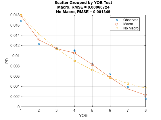
Figure contains an axes object. The axes object with title Scatter Grouped by YOB Test Macro, RMSE = 0.00060724 No Macro, RMSE = 0.001349, xlabel YOB, ylabel PD contains 3 objects of type line. One or more of the lines displays its values using only markers These objects represent Observed, Macro, No Macro.

modelCalibrationPlot(ModelMacro,data(Ind,:),{'YOB','ScoreGroup'},'ReferencePD',data.PDNoMacro(Ind),'ReferenceID',ModelNoMacro.ModelID,'DataID',DataSetChoice)

The accuracy of the predictions significantly improves compared to the model with no macroeconomic variables. The predicted conditional PD values more closely follow the pattern of the observed default rates and the root mean square error (RMSE) reported is significantly smaller when the macroeconomic variables are included in the model.

Plot the ROC curve of the macro model and the model without macroeconomic variables to compare their performance with regards to model discrimination.

modelDiscriminationPlot(ModelMacro,data(Ind,:),'ReferencePD',data.PDNoMacro(Ind),'ReferenceID',ModelNoMacro.ModelID,'DataID',DataSetChoice)

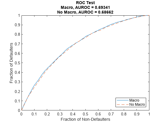
Figure contains an axes object. The axes object with title ROC Test Macro, AUROC = 0.69341 No Macro, AUROC = 0.68662, xlabel Fraction of Non-Defaulters, ylabel Fraction of Defaulters contains 2 objects of type line. These objects represent Macro, No Macro.

Discrimination measures the ranking of customers by risk. Both models perform similarly, with only a slight improvement when the macroeconomic variables are added to the model. This means both models do a similar job separating low risk, medium risk and high risk customers by assigning higher PD values to customers with higher risk.

Although the discrimination performance of both models is similar, the predicted PD values are more accurate for the macro model. Using both discrimination and accuracy tools is important for model validation and model comparison.

Stress Testing of Probability of Default

Use the fitted macro model to stress-test the predicted probabilities of default.

Assume the following are stress scenarios for the macroeconomic variables provided, for example, by a regulator.

disp(dataMacroStress)

                 GDP     Market
                _____    ______

    Baseline     2.27    15.02 
    Adverse      1.31     4.56 
    Severe      -0.22    -5.64

Set up a basic data table for predicting the probabilities of default. This is a dummy data table, with one row for each combination of score group and number of years on books.

dataBaseline = table;
[ScoreGroup,YOB]=meshgrid(1:NumScoreGroups,1:NumYOB);
dataBaseline.ScoreGroup = categorical(ScoreGroup(:),1:NumScoreGroups,...
   categories(data.ScoreGroup),'Ordinal',true);
dataBaseline.YOB = YOB(:);
dataBaseline.ID = ones(height(dataBaseline),1);
dataBaseline.GDP = zeros(height(dataBaseline),1);
dataBaseline.Market = zeros(height(dataBaseline),1);

To make the predictions, set the same macroeconomic conditions (baseline, adverse, or severely adverse) for all combinations of score groups and number of years on books.

% Predict baseline the probabilities of default
dataBaseline.GDP(:) = dataMacroStress.GDP('Baseline');
dataBaseline.Market(:) = dataMacroStress.Market('Baseline');
dataBaseline.PD = predict(ModelMacro,dataBaseline);

% Predict the probabilities of default in the adverse scenario
dataAdverse = dataBaseline;
dataAdverse.GDP(:) = dataMacroStress.GDP('Adverse');
dataAdverse.Market(:) = dataMacroStress.Market('Adverse');
dataAdverse.PD = predict(ModelMacro,dataAdverse);

% Predict the probabilities of default in the severely adverse scenario
dataSevere = dataBaseline;
dataSevere.GDP(:) = dataMacroStress.GDP('Severe');
dataSevere.Market(:) = dataMacroStress.Market('Severe');
dataSevere.PD = predict(ModelMacro,dataSevere);

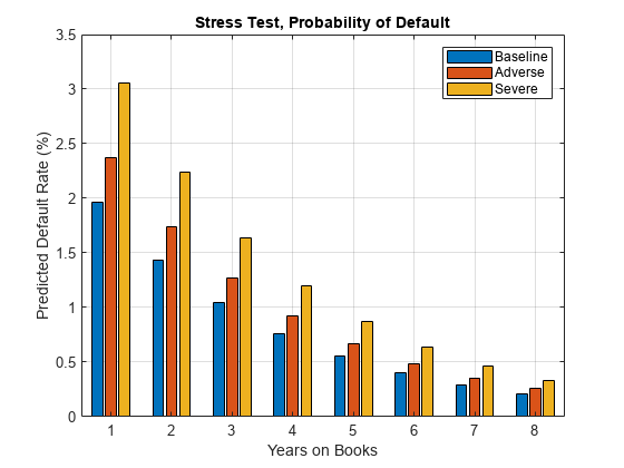
Visualize the average predicted probability of default across score groups under the three alternative regulatory scenarios. Here, all score groups are implicitly weighted equally. However, predictions can also be made at a loan level for any given portfolio to make the predicted default rates consistent with the actual distribution of loans in the portfolio. The same visualization can be produced for each score group separately.

PredPDYOB = zeros(NumYOB,3);
PredPDYOB(:,1) = mean(reshape(dataBaseline.PD,NumYOB,NumScoreGroups),2);
PredPDYOB(:,2) = mean(reshape(dataAdverse.PD,NumYOB,NumScoreGroups),2);
PredPDYOB(:,3) = mean(reshape(dataSevere.PD,NumYOB,NumScoreGroups),2);

figure;
bar(PredPDYOB*100);
xlabel('Years on Books')
ylabel('Predicted Default Rate (%)')
legend('Baseline','Adverse','Severe')
title('Stress Test, Probability of Default')
grid on

Figure contains an axes object. The axes object with title Stress Test, Probability of Default, xlabel Years on Books, ylabel Predicted Default Rate (%) contains 3 objects of type bar. These objects represent Baseline, Adverse, Severe.