envspectrum

Simulate two vibration signals, one from a healthy bearing and one from a damaged bearing. Compute and compare their envelope spectra.

A bearing with a pitch diameter of 12 cm has eight rolling elements. Each rolling element has a diameter of 2 cm. The outer race remains stationary as the inner race is driven at 25 cycles per second. An accelerometer samples the bearing vibrations at 10 kHz.

fs = 10000;
f0 = 25;
n = 8;
d = 0.02;
p = 0.12;

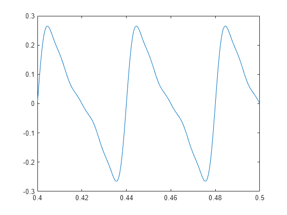
The vibration signal from the healthy bearing includes several orders of the driving frequency. Plot 0.1 second of data.

t = 0:1/fs:1-1/fs;
z = [1 0.5 0.2 0.1 0.05] ...
    *sin(2*pi*f0*[1 2 3 4 5]'.*t)/5;

plot(t,z)
xlim([0.4 0.5])

A defect in the outer race of the bearing causes a series of 5 millisecond impacts on the bearing. Eventually, those impacts result in bearing wear. The impacts occur at the ball pass frequency outer race (BPFO) of the bearing,

where $$f_0$$ is the driving rate, n is the number of rolling elements, d is the diameter of the rolling elements, p is the pitch diameter of the bearing, and θ is the bearing contact angle. Assume a contact angle of zero and compute the BPFO.

ca = 0;
bpfo = n*f0/2*(1-d/p*cos(ca))

bpfo = 
83.3333

Model the impacts as a periodic train of 3 kHz sinusoids windowed by a flat top window. Plot 0.1 second of data.

fImpact = 3000;
tImpact = 0:1/fs:5e-3-1/fs;
xImpact = sin(2*pi*fImpact*tImpact)...
    .*flattopwin(length(tImpact))'/10;

x = pulstran(t,0:1/bpfo:t(end),xImpact,fs)/3;

plot(t,x+z)
xlim([0.4 0.5])

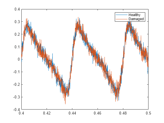
Add white Gaussian noise to the signals. Specify a noise variance of 1/30². Plot 0.1 second of data.

yGood = z + randn(size(z))/30;
yBad = x+z + randn(size(z))/30;
plot(t,yGood,t,yBad)
xlim([0.4 0.5])
legend("Healthy","Damaged")

Compute and plot the envelope signals and spectra.

envspectrum([yGood' yBad'],fs)
xlim([0 10*bpfo]/1000)

Compare the peak locations to the frequencies of harmonics of the BPFO. The BPFO harmonics in the envelope spectrum are a sign of bearing wear.

harmImpact = (1:10)*bpfo;
xline(harmImpact/1000,":")
legend("Healthy","Damaged","BPFO harmonics")

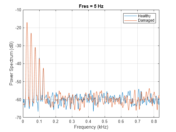
Compute the Welch spectra of the signals. Specify a frequency resolution of 5 Hz.

figure
pspectrum([yGood' yBad'],fs,FrequencyResolution=5)
legend("Healthy","Damaged")

At the low end of the spectrum, the driving frequency and its orders obscure other features. The spectrum of the healthy bearing and the spectrum of the damaged bearing are indistinguishable.

xlim([0 10*bpfo]/1000)

The spectrum of the faulty bearing shows BPFO harmonics modulated by the impact frequency.

xlim((bpfo*[-10 10]+fImpact)/1000)

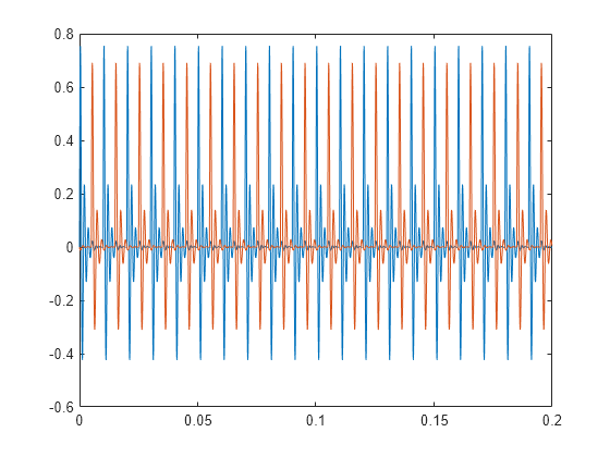
Generate a two-channel signal that resembles the vibration signals from a bearing that completes a rotation every 10 milliseconds. The signal is sampled at 10 kHz for 0.2 seconds, which corresponds to 20 bearing rotations.

fs = 10000;
tmax = 20;
mlt = 0.01;
t = 0:1/fs:mlt-1/fs;

During each 10-millisecond interval:

Plot the signal.

y1 = sin(2*pi*600*t).*exp(-700*t);
y2 = sin(2*pi*500*t).*exp(-800*t);
y2 = [y2(51:100) y2(1:50)];

T = (0:1/fs:mlt*tmax-1/fs)';
Y = repmat([y1;y2],1,tmax)';

plot(T,Y)

Create a duration array using the time interval T. Construct a timetable with the duration array and the two-channel signal.

dt = seconds(T);
ttb = timetable(dt,Y);

Use envspectrum with no output arguments to display the envelope signal and envelope spectrum of the two channels. Compute the spectrum on the whole Nyquist interval, excluding 100 Hz intervals at the ends.

envspectrum(ttb,'Band',[100 4900])

The envelope spectra of the signals have peaks at integer multiples of the repetition rate of 1/0.01 = 0.1 kHz. This is just as expected. envspectrum removes the high-frequency sinusoidal components and focuses on the lower-frequency repetition behavior. This is why the envelope spectrum is a useful tool for the analysis of rotational machinery.

Compute the envelope signal and the times at which it is computed. Check the types of the output variables.

[~,~,ttbenv,ttbt] = envspectrum(ttb,'Band',[100 4900]);
whos ttb*

  Name           Size            Bytes  Class        Attributes

  ttb         2000x1             48977  timetable              
  ttbenv      2000x1             48985  timetable              
  ttbt        2000x1             16002  duration               

The time vector is of duration type, like the time values of the input timetable. The output timetable has the same size as the input timetable.

Store each channel of the input timetable as a separate variable. Compute the envelope signal and the time vector. Check the output types.

btb = timetable(dt,Y(:,1),Y(:,2));

[~,~,btbenv,btbt] = envspectrum(btb,'Band',[100 4900]);
whos btb*

  Name           Size            Bytes  Class        Attributes

  btb         2000x2             49231  timetable              
  btbenv      2000x2             49251  timetable              
  btbt        2000x1             16002  duration               

The output timetable has the same size as the input timetable.

Generate a signal sampled at 1 kHz for 5 seconds. The signal consists of 0.01-second rectangular pulses that repeat every T = 0.25 second. Amplitude modulate the signal onto a sinusoid of carrier frequency 150 Hz.

fs = 1e3;
tmax = 5;

t = 0:1/fs:tmax;
y = pulstran(t,0:0.25:tmax,rectpuls=0.01);

fc = 150;
z = modulate(y,fc,fs);

Plot the original and modulated signals. Show only the first few cycles.

plot(t,y,t,z,"-")
grid on
axis([0 1 -1.1 1.1])

Compute the envelope and envelope spectrum of the signal. Determine the signal envelope using complex demodulation. Compute the envelope spectrum on a 20 Hz interval centered at the carrier frequency.

[q,f,e,te] = envspectrum(z,fs,Method="demod",Band=[fc-10 fc+10]);

Plot the envelope signal and the envelope spectrum. Zoom in on the interval from 0 to 50 Hz.

subplot(2,1,1)
plot(te,e)
xlabel("Time")
title("Envelope")

subplot(2,1,2)
plot(f,q)
xlim([0 50])
xlabel("Frequency")
title("Envelope Spectrum")

The envelope signal has the same period in time, T = 0.25 second, as the original signal. The envelope spectrum has pulses at 1 / T = 4 Hz.

Repeat the computation, but now use the hilbert function to compute the envelope. Bandpass-filter the signal using a 10th-order finite impulse response (FIR) filter. Plot the envelope signal and envelope spectrum using the built-in functionality of envspectrum.

envspectrum(z,fs,Method="hilbert",FilterOrder=10)

Embed the signal in white Gaussian noise of variance 1/3. Plot the result.

zn = z + randn(size(z))/3;

plot(t,zn,"-")
grid on
axis([0 1 -1.1 1.1])

Compute and display the envelope signal and envelope spectrum. Compute the envelope spectrum using complex demodulation on a 10 Hz interval centered at the carrier frequency. Zoom in on the interval from 0 to 50 Hz.

envspectrum(zn,fs,Band=[fc-5 fc+5])
xlim([0 50])