Adaptive Notch Filter
Automatically adjust notch filter parameters based on detected resonance
Since R2026a
Libraries:
Simulink Control Design /
Adaptive Control
Description
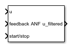
The Adaptive Notch Filter block automatically adjusts the notch frequency, depth, and width to filter resonances as well as any other frequency of interest such as harmonics or sideband frequencies. To perform adaptive notch filtering, the block provides two methods:
| Method | When to Use | Adaptation Summary |
|---|---|---|
| Identify and remove system resonances | You want to identify the slowly varying resonant frequency using frequency‑response estimation, and suppress it with the adaptive notch filter. |
|
| Remove content at single frequency | You want to continuously apply adaptive notch filtering to a specified frequency or to the highest peak in the input spectrum. You can also use this configuration for resonances, but is more general purpose and is mostly helpful for power systems or electrical applications to just remove a single arbitrary frequency |
|
The algorithms used are summarized as follows:
Frequency Response Estimation — The algorithm simultaneously injects perturbation signals into the plant at the nominal operating point, collects response data from the plant output, and computes the estimated frequency response. For more information, see Frequency Response Estimator.
Peak Detection — The peak detection algorithm scans the magnitude spectrum using a sliding window and identifies local maxima based on absolute and relative thresholds. It checks whether the center point in the window is larger than the points on either side and satisfies threshold conditions. The algorithm stores valid peaks and selects the highest one as the resonant frequency.
Goertzel Algorithm — The Goertzel algorithm computes the DFT at a single frequency bin by running a simple recursive filter over a block of N input samples. It tracks the signal energy at the chosen frequency and outputs the real and imaginary components needed to compute magnitude and phase. The algorithm updates this estimate each sliding window and uses a moving average to smooth noise in the magnitude output.
Adaptation Algorithm — ESC adjusts the notch filter width and depth in real time to reduce the controller input error. It uses the mean-squared error (MSE), which measures the squared error entering the PID controller and highlights energy at the resonant frequency. ESC processes this MSE through an objective function and updates the notch filter so the error moves toward zero. So, MSE identifies the unwanted resonance, and ESC continuously adapts the filter to suppress it.
For the computed parameters, the block uses a Tustin discretization of the instantaneous transfer function of the filter is given by:
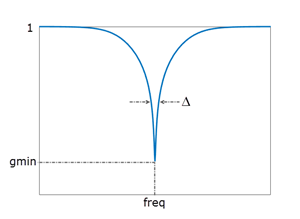
where gmin, damp, and freq are the values obtained by adapting the notch parameters. These parameters control the notch depth and frequency as shown in the following illustration. The damping ratio damp controls the notch width Δ; larger damp means larger Δ.
Examples
This example shows how to configure the Adaptive Notch Filter (ANF) block to perform filtering based on the frequency response estimation (FRE) of the plant. In this mode, the block first estimates the frequency response of the plant and identifies the peak location. Then, enables the adaptation algorithm for identifying the notch width and depth parameters. This is helpful when you have slowly-varying resonances. Once the block identifies a peak, the location of the notch does not change. If your resonance location changes, you must trigger FRE again to find the new peak.
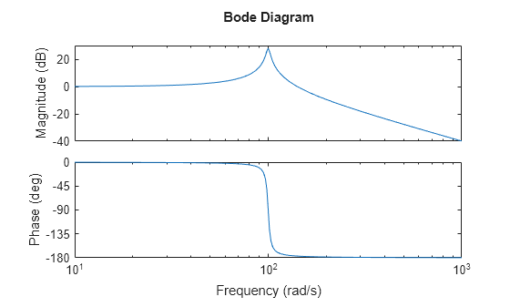
The Simulink® model anfFRE.slx, provided with this example, shows the simplest way you can use the ANF block to filter based on the identified resonance from the estimated frequency response. For this example, use transfer function of a plant with resonance at 100 rad/s.
H = tf(10000,[1 4 10000]);
H = c2d(H,0.001,"matched");
bodeplot(H,{1 1e3})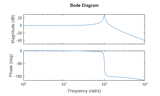
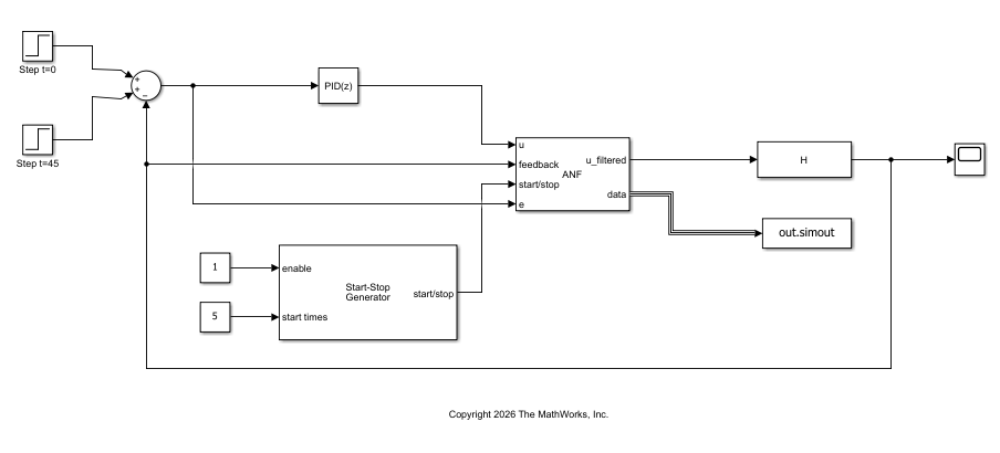
[C,info] = pidtune(H,"PID",30);The model is configured to simulate a step response at 0 s to bring the closed loop-system to a nominal operating. Between 5 and 40 seconds, the ANF block performs frequency response estimation of the plant by injecting perturbation signals. After the FRE converges and block identifies the resonance location, it starts the adaptation algorithm. The second step occurs at 45 seconds, which is the filtered output. In this configuration, the input u of the ANF block is connected to the input to the plant (controller output), feedback to the plant output , and start/stop signal enables and disables the FRE experiment. Open the model.
mdl = "anfFRE";
open_system(mdl)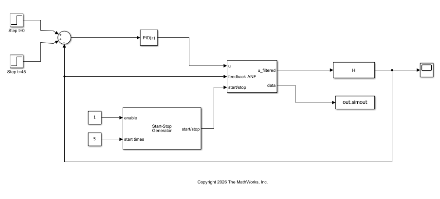
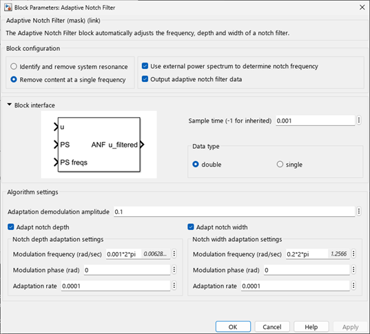
The block in this model adapts both the notch depth and width based on the identified resonance. The following image shows how the block is configured.
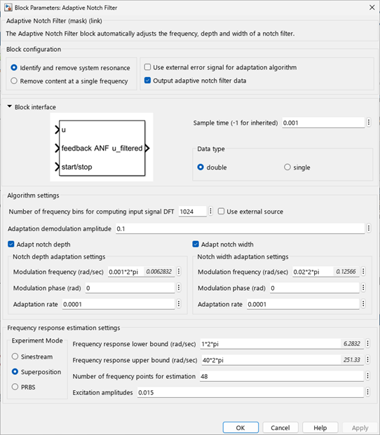
Simulate the model.
out = sim(mdl);
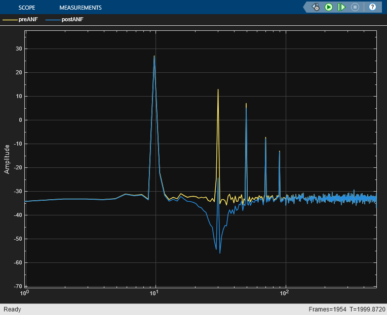
open_system(mdl+"/Scope")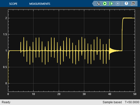
In the initial value the signals do not differ as the entire power spectrum is not estimated yet. After the step occurs at 15 seconds, the ANF block successfully attenuates the resonant peak and the filtered response does not exhibits large oscillations.
The ANF block data port outputs the notch parameters over each time step. For example, verify the accuracy of estimated frequency response. The estimated frequency response and the identified peak closely matches the original response.
wr = out.simout.notchFreq.Data(end) % Peakwr = 100.0053
resp = out.simout.freFRD.Data;
fsys = frd(squeeze(resp(end,:)),linspace(1*2*pi,40*2*pi,48),0.001);
bodeplot(H,fsys,"r--",{1 1e3})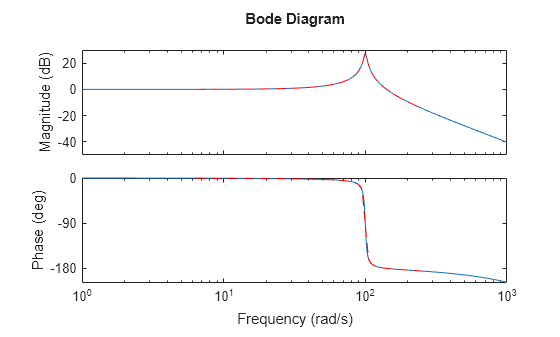
Use the logged data to check the convergence of the notch filter parameters.
figure
tiledlayout("flow")
nexttile
plot(out.simout.notchDepth.Time,squeeze(out.simout.notchDepth.Data))
nexttile
plot(out.simout.notchWidth.Time,squeeze(out.simout.notchWidth.Data))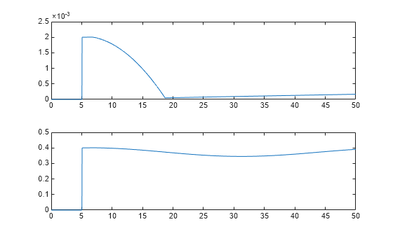
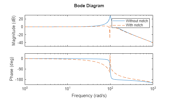
You can also use the values to create an LTI model of the notch filter and validate results for the converged values. Since the model H, is in discrete time, convert the notch filter to match the time domain.
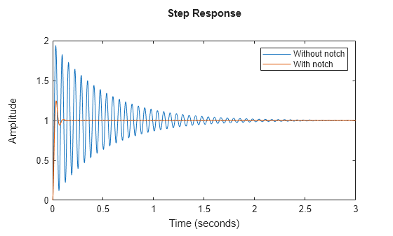
gmin = out.simout.notchDepth.Data(end); % Depth
damp = out.simout.notchWidth.Data(end); % Width
H_notch = tf([1 (2*gmin*damp*wr) (wr^2)], [1 (2*damp*wr) (wr^2)]);
H_notch = c2d(H_notch,0.001,"tustin");
figure
bodeplot(C*H,C*H_notch*H,"--",{1 1e3})
legend("Without notch","With notch",Location="best")
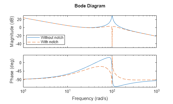
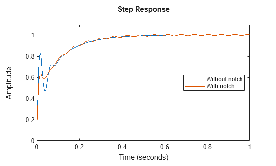
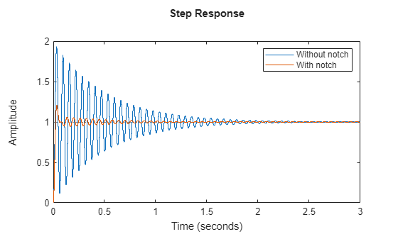
figure
stepplot(feedback(C*H,1),feedback(C*H*H_notch,1),1);
legend("Without notch","With notch",Location="best")
In this configuration, you can also supply the error signal from an upstream controller (such as PID) directly at the block input e. This is helpful when you have more complex control structures and want to use external error for adaptation.
This example shows how to configure the Adaptive Notch Filter (ANF) block to perform filtering at a known single frequency. In this mode, the block continuously adapts the notch width and depth parameters at the single given frequency. This is helpful when you want to filter a fixed frequency.
The Simulink® model anfSingleFrequency.slx, provided with this example, shows the simplest way you can use the ANF block to filter a single frequency. For this example, use transfer function of a plant with resonance at 100 rad/s. The example shows how to filter a resonance at this given frequency, but this configuration is more general purpose and is mostly meant for power systems or electrical applications to just remove a single arbitrary frequency.
H = tf(10000,[1 4 10000]);
bode(H)
The model is configured to simulate a step response of the filtered and unfiltered plant output. In this configuration, the input u of the ANF block is connected to the signal you want to filter and f is connected to the frequency at which the resonance occurs. Open the model.
mdl = "anfSingleFrequency";
open_system(mdl)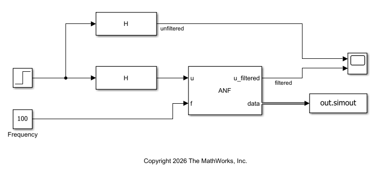
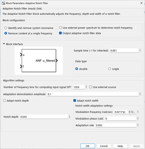
The Adaptive Notch Filter takes the input signal to filter and adapts notch width and depth value based on the characteristics of the frequency. The block in this model uses a fixed depth value and adapts the notch width.
Simulate the model and display the unfiltered and filtered step response of the transfer function.
out = sim(mdl);
open_system(mdl+"/Scope")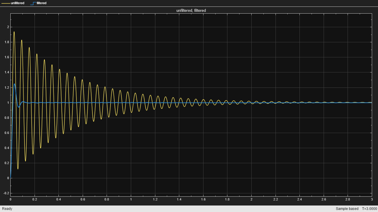
The ANF block successfully attenuates the resonant peak and the filtered response does not exhibits large oscillations.
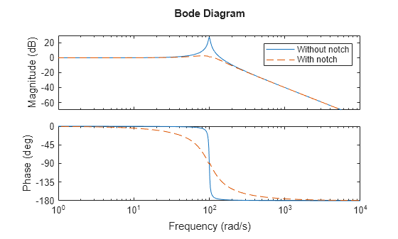
The ANF block data port outputs the notch parameters over each time step. For example, you can use the values to create an LTI model of the notch filter and validate results for the converged values.
gmin = out.simout.notchDepth.Data(end); % Depth
damp = out.simout.notchWidth.Data(end); % Width
wr = out.simout.notchFreq.Data(end);    % Frequency
H_notch = tf([1 (2*gmin*damp*wr) (wr^2)], [1 (2*damp*wr) (wr^2)]);
bode(H,H*H_notch,"--")
legend("Without notch","With notch")
step(H,H*H_notch,3);
legend("Without notch","With notch")
Copyright 2025 The MathWorks, Inc
This example shows how to configure the Adaptive Notch Filter (ANF) block to perform filtering based on a power spectrum of the signal to filter. In this mode, the block continuously adapts the notch width and depth parameters based on the power spectrum of the signal. This is helpful when you have a power spectrum from an external source, such as a Spectrum Estimator block, and want to continuously perform filtering.
The Simulink® model anfPowerSpectrum.slx, provided with this example, shows the simplest way you can use the ANF block to filter based on the power spectrum input. For this example, use transfer function of a plant with resonance at 100 rad/s.
H = tf(10000,[1 4 10000]);
H = c2d(H,0.001,"matched");
bode(H,{1 1e3})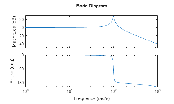
The model is configured to simulate a step response of the filtered and unfiltered plant output. The initial value of the Step block is set to 1 and the step occurs at 15 seconds. In this configuration, the input u of the ANF block is connected to the signal you want to filter, and PS and PS freqs are connected to the power spectrum and corresponding frequencies (in rad/s), obtained using the Spectrum Estimator block. Open the model.
mdl = "anfPowerSpectrum";
open_system(mdl)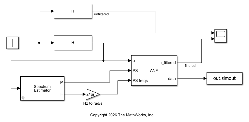
The Adaptive Notch Filter takes the input signal to filter and adapts notch width and depth value based on the resonant peak magnitude and location determined from the power spectrum. The block in this model adapts both the notch depth and width.
Simulate the model and display the unfiltered and filtered step response of the transfer function.
out = sim(mdl);
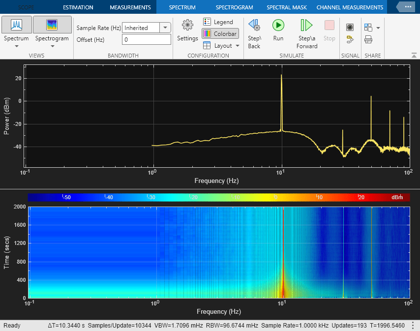
open_system(mdl+"/Scope")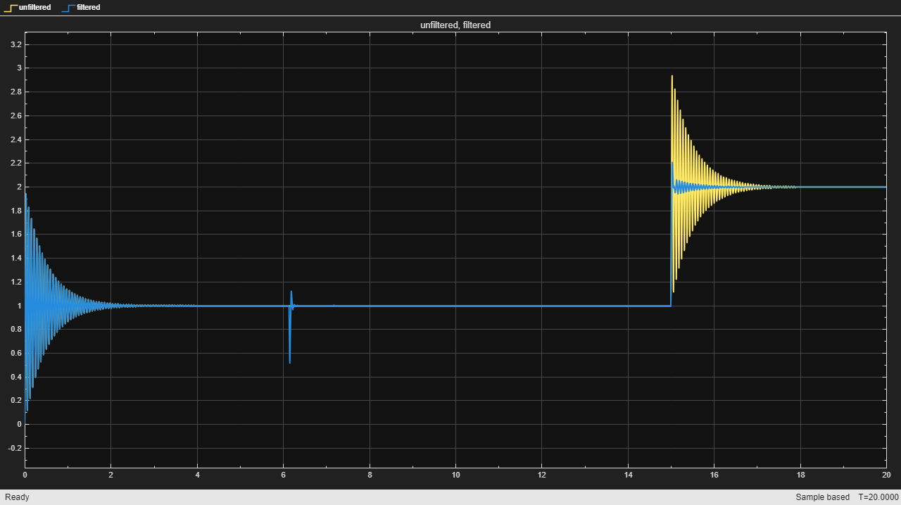
In the initial value the signals do not differ as the entire power spectrum is not estimated yet. After the step occurs at 15 seconds, the ANF block successfully attenuates the resonant peak and the filtered response does not exhibits large oscillations.
The ANF block data port outputs the notch parameters over each time step. For example, you can use the values to create an LTI model of the notch filter and validate results for the converged values. Since the model H, is in discrete time, convert the notch filter to match the time domain.
gmin = out.simout.notchDepth.Data(end); % Depth
damp = out.simout.notchWidth.Data(end); % Width
wr = out.simout.notchFreq.Data(end);    % Frequency
H_notch = tf([1 (2*gmin*damp*wr) (wr^2)], [1 (2*damp*wr) (wr^2)]);
H_notch = c2d(H_notch,0.001,"tustin");
bode(H,H*H_notch,"--",{1 1e3})
legend("Without notch","With notch")
step(H,H*H_notch,3);
legend("Without notch","With notch")
This example shows how to filter a harmonic using the Adaptive Notch Filter (ANF) block based on a power spectrum of the signal to filter. The Simulink® model anfHarmonics.slx, provided with this example, shows the simplest way you can use the ANF block to filter harmonics based on the power spectrum input. The generates harmonics applied to a fundamental frequency and filters out the third harmonic.
Open the model.
mdl = "anfHarmonics";
open_system(mdl)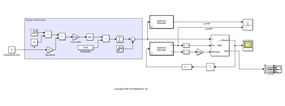
The model is configured to select the third harmonic based on the estimated power spectrum of the signal, and filter it out. The ANF block adapts the notch based on the detected magnitude from the spectrum.
Simulate the model.
sim(mdl);
Extended Examples

Suppress PMSM Harmonics Using Adaptive Notch Filter
Reduce harmonic distortion in a PMSM using an extremum seeking control based adaptive notch filter.

Suppress Resonances Using Adaptive Notch Filter
Suppress resonances in a coupled inertia system using an adaptive notch filter implement using extremum seeking control and frequency response estimator.
Ports
Input
Output
Parameters
Extended Capabilities
Version History
Introduced in R2026a