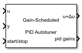
Gain-Scheduled PID Autotuner
Libraries:
Simulink Control Design /
Autotuning
Description
Use the new Gain-Scheduled PID Autotuner block from the Autotuning library to automatically tune PID gains at multiple operating points based on plant frequency responses estimated from closed-loop experiment. The tuning workflow is similar to the Closed-Loop PID Autotuner block, and the block allows you to specify additional options to set up gain scheduling such as breakpoints and scheduling variable. The block performs tuning sequentially for each operating point. When autotuning is complete, the block allows you to store and look up the PID gain values based on the scheduling variable and breakpoint data and write them to the PID controller without stopping the simulation.
Examples
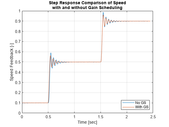
This example shows how to validate the gain-scheduled autotuning results for a water tank model. The model is preconfigured to tune gain-scheduled controller gains at four operating points.
Open the model.
Kp = 1.599340;
Ki = 0.079967;
mdl = "watertankGSAuto"
mdl = "watertankGSAuto"

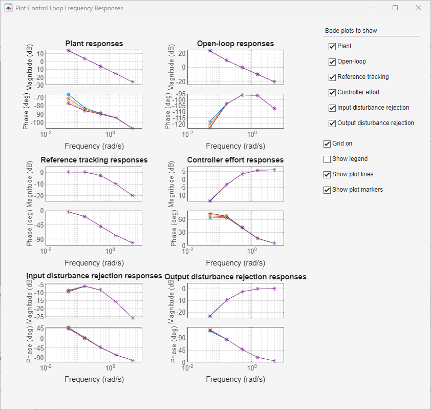
During the tuning process, you can select to display Bode plots of control loop responses and gain surface to validate results.
Simulate the model.
sim(mdl);
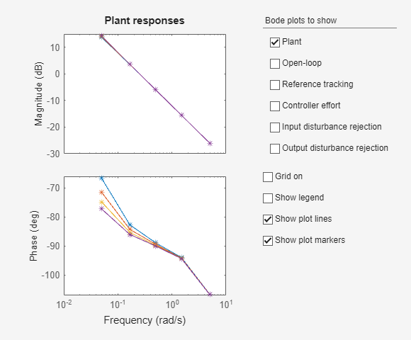
By default, the block displays the estimated plant frequency response. You can plot additional responses using the Bode plots to show options.
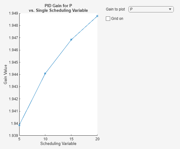
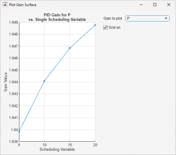
Additionally, you can visualize the gain values at each value of the scheduling variable.
Extended Examples
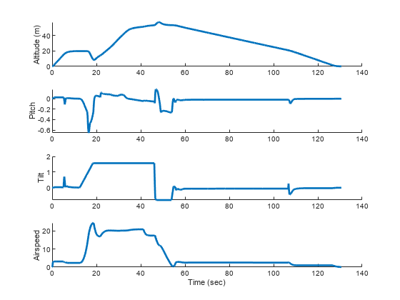
Gain-Scheduled PID Autotuning a VTOL UAV During Forward and Backward Transition
Tune gain-scheduled PID controller for VTOL UAV transitioning between operating modes.
- Since R2024a
- Open Live Script
Gain-Scheduled PID Autotuning Torque Control for a Nonlinear PMSM
Tune gain-scheduled PID controllers for d-axis and q-axis current loops of a nonlinear PMSM model.
- Since R2024a
- Open Live Script
Ports
Input
Insert the block into your system such that this port accepts a control signal from a source. Typically, this port accepts the signal from the PID controller in your system.
Data Types: single | double
Connect this port to the plant output.
Data Types: single | double
To start and stop the autotuning process, provide a signal at the
start/stop port. When the value of the signal changes
from:
Negative or zero to positive, the experiment starts
Positive to negative or zero, the experiment stops
When the experiment is not running, the block passes signals unchanged from u to u+Δu. In this state, the block has no impact on plant or controller behavior.
Typically, you can use a signal that changes from 0 to 1 to start the experiment, and from 1 to 0 to stop it. Some points to consider when configuring the start/stop signal include:
Start the experiment when the plant is at the desired equilibrium operating point. Use the initial controller to drive the plant to the operating point. If you have no initial controller (open-loop tuning only) you can use a source block connected to u to drive the plant to the operating point.
Avoid any load disturbance to the plant during the experiment. Load disturbance can distort the plant output and reduce the accuracy of the frequency-response estimation.
Let the experiment run long enough for the algorithm to collect sufficient data for a good estimate at all frequencies it probes.
For Sinestream and Superposition modes, there are two ways to determine when to stop the experiment:
Determine the experiment duration in advance. A conservative estimate for the experiment duration is 200/ωc in superposition experiment mode or 550/ωc in sinestream experiment mode, where ωc is your target bandwidth.
Observe the signal at the
% convoutput, and stop the experiment when the signal stabilizes near 100%.
For PRBS mode, based on the specified Target bandwidth and Controller sample time values, the block dialog box displays the recommended experiment length in the Description section of the Experiment tab. Stopping experiment prematurely may lead to incorrect tuning results.
When you stop the experiment, the block computes tuned PID gains and updates the signal at the
pid gainsport.
You can configure any logic appropriate for your application to control the start and stop times of the experiment.
Data Types: single | double
Supply a value for the Target bandwidth (rad/sec) parameter.
See that parameter for details.
Dependencies
To enable this port, in the Autotuner tab, next to
Target bandwidth (rad/sec), select Use external
source.
Data Types: single | double
Supply a value for the Target phase margin (degrees)
parameter. See that parameter for details.
Dependencies
To enable this port, in the Autotuner tab, next to
Target phase margin (degrees), select Use external
source.
Data Types: single | double
Supply a value for the Signal Amplitudes parameter. See that
parameter for details.
Dependencies
To enable this port, in the Autotuner tab, next to
Signal Amplitudes, select Use external
source.
Data Types: single | double
Specify the scheduling variable. This signal indicates where in the operating range the system is at a given time. The lookup tables use this signal to determine the value of the PID gains.
Since R2026a
Specify the second scheduling variable. This signal indicates where in the operating range the system is at a given time. The lookup tables uses these scheduling variables signal to determine the value of the PID gains.
Dependencies
To enable this port, in the Gain scheduling tab, select Use two scheduling variables.
Breakpoint data for first scheduling variable, specified as a vector.
Dependencies
To enable this port, select Use external signal.
Since R2026a
Breakpoint data for second scheduling variable, specified as a vector.
Dependencies
To enable this port, select Use two scheduling variables and Use external signal.
Control signal to trigger the update of gains.
Dependencies
To enable this port, set Method to trigger gain update to External trigger.
Output
Insert the block into your system such that this port feeds the input signal to your plant.
When the experiment is running (
start/stoppositive), the block injects test signals into the plant at this port. If you have any saturation or rate limit protecting the plant, feed the signal from u+Δu into it.When the experiment is not running (
start/stopzero or negative), the block passes signals unchanged from u to u+Δu.
Dependencies
To enable this port, in Output Signal Configuration, select control + perturbation.
Data Types: single | double
The block generates a perturbation signal at this port. Typically, you inject the perturbation from this port via a sum block.
When the experiment is running (start/stop positive), the block generates perturbation signals at this port.
When the experiment is not running (start/stop zero or negative), the signal at this port is zero. In this state, the block has no effect on the plant.
Dependencies
To enable this port, in Output Signal Configuration, select perturbation only.
Data Types: single | double
This 4-element bus signal contains the tuned PID gains P,
I, D, and the filter coefficient
N. These values correspond to the P,
I, D, and N parameters in
the expressions given in the Form parameter. Initially, the
values are 0, 0, 0, and 100, respectively. The block updates the values when the
experiment ends. This bus signal always has four elements, even if you are not tuning
a PIDF controller.
Data Types: single | double
This port outputs the estimated phase margin achieved by the tuned controller, in
degrees. The block updates this value when the tuning experiment ends. The estimated
phase margin is calculated from the angle of
G(jωc)C(jωc),
where G is the estimated plant, C is the tuned
controller, and ωc is the crossover
frequency (bandwidth). The estimated phase margin might differ from the target phase
margin specified by the Target phase margin (degrees) parameter.
It is an indicator of the robustness and stability achieved by the tuned
system.
Typically, the estimated phase margin is near the target phase margin. In general, the larger the value, the more robust is the tuned system, and the less overshoot there is.
A negative phase margin indicates that the closed-loop system might be unstable.
Dependencies
To enable this port, in the Tuning tab, select Output estimated phase margin achieved by tuned controller.
This port outputs the frequency-response data estimated by the experiment.
Initially, the value at frd is [0, 0, 0, 0, 0]. During the
experiment, the block injects signals at frequencies [1/10, 1/3, 1, 3,
10]ωc, where ωc is the target
bandwidth. At each sample time during the experiment, the block updates
frd with a vector containing the complex frequency response at
each of these frequencies, respectively. For sinestream and superposition signals, you
can use the progress of the response as an alternative to % conv
to examine the convergence of the estimation. When the experiment stops, the block
updates frd with the final estimated frequency response used for
computing the PID gains.
For PRBS experiment mode, the signal at this port updates only after the estimation experiment has finished.
Dependencies
To enable this port, in the Experiment tab, select Plant frequency responses near bandwidth.
Parameters
To edit block parameters interactively, use the Property Inspector. From the Simulink® Toolstrip, on the Simulation tab, in the Prepare gallery, select Property Inspector.
Controller Settings
Specify the type of the PID controller in your system. The controller type indicates what actions are present in the controller. The following controller types are available for PID autotuning:
P— Proportional onlyI— Integral onlyPI— Proportional and integralPD— Proportional and derivativePDN— Proportional and derivative with derivative filterPID— Proportional, integral, and derivativePIDN— Proportional, integral, and derivative with derivative filter
The controller type must match the PID controller you are tuning.
Specify the controller form. The controller form determines the interpretation of the PID coefficients P, I, D, and N.
Parallel— InParallelform, the transfer function of a discrete-time PIDF controller is:where Fi(z) and Fd(z) are the integrator and filter formulas (see
Integrator methodandFilter method). The transfer function of a continuous-time parallel-form PIDF controller is:Other controller actions amount to setting P, I, or D to zero.
Ideal— InIdealform, the transfer function of a discrete-time PIDF controller is:The transfer function of a continuous-time ideal-form PIDF controller is:
Other controller actions amount to setting D to zero or setting, I to
Inf. (In ideal form, the controller must have proportional action.)
The controller form must match the PID controller you are tuning.
Tunable: Yes
Specify the sample time of your PID controller in seconds. This value also sets the sample time for the experiment performed by the block.
To perform PID tuning, the block measures frequency-response information up to a frequency of 10 times the target bandwidth. To ensure that this frequency is less than the Nyquist frequency, the target bandwidth, ωc, must satisfy ωcTs ≤ 0.3, where Ts ωc is the controller sample time that you specify with the Sample time parameter.
When you update a PID Controller block or custom PID controller with tuned parameter values, make sure the controller sample time matches.
Tips
If you want to run the deployed block with different sample times in your application, set this parameter to –1 and put the block in a Triggered Subsystem. Then, trigger the subsystem at the desired sample time. If you do not plan to change the sample time after deployment, specify a fixed and finite sample time.
Specify the floating-point precision based on simulation environment or hardware requirements.
Autotuner Tab
Enable this parameter to run tuning at a sample rate that is different from the sample rate of the PID controller you are tuning and the frequency response estimation experiment performed by the block. The PID gain tuning algorithm is computationally intensive, and when you want to deploy the block to hardware and tune a controller with a fast sample time, some hardware might not complete the PID gain calculation in a single time step. To reduce the hardware throughput requirements, specify a tuning sample time slower than the controller sample time using the Tuning sample time parameter.
Specify the sample time of the tuning algorithm in seconds.
If you intend to deploy the block on hardware with limited processing power and want to tune a controller with a fast sample time, specify a sample time such that the tuning algorithm runs at a slower rate than the PID controller you are tuning.
Dependencies
To enable this parameter, select Tune at different sample time.
Specify the discrete integration formula for the integrator term in your controller. In discrete time, the PID controller transfer function assumed by the block is:
in parallel form, or in ideal form,
For a controller sample time Ts, the
Integrator method parameter determines the formula
Fi as follows:
| Integrator method | Fi |
|---|---|
Forward Euler |
|
Backward Euler |
|
Trapezoidal |
|
For more information about the relative advantages of each method, see the Discrete PID Controller block reference page.
Tunable: Yes
Specify the discrete integration formula for the derivative filter term in your controller. In discrete time, the PID controller transfer function assumed by the block is:
in parallel form, or in ideal form,
For a controller sample time Ts, the
Filter method parameter determines the formula
Fd as follows:
| Filter method | Fd |
|---|---|
Forward Euler |
|
Backward Euler |
|
Trapezoidal |
|
For more information about the relative advantages of each method, see the Discrete PID Controller block reference page.
Tunable: Yes
The target bandwidth, specified in rad/sec, is the target value for the 0-dB gain crossover frequency of the tuned open-loop response CP, where P is the plant response, and C is the controller response. This crossover frequency roughly sets the control bandwidth. For a rise-time τ seconds, a good guess for the target bandwidth is 2/τ rad/sec.
To perform PID tuning, the autotuner block measures frequency-response information up to a frequency of 10 times the target bandwidth. To ensure that this frequency is less than the Nyquist frequency, the target bandwidth, ωc, must satisfy ωcTs ≤ 0.3, where Ts is the controller sample time that you specify with the Sample time parameter. Because of this condition, the fastest rise time you can enforce for tuning is about 6.67Ts. If this rise time does not meet your design goals, consider reducing Ts.
For best results with closed-loop tuning, use a target bandwidth that is within about a factor of 10 of the bandwidth with the initial PID controller. To tune a controller for a larger change in bandwidth, tune incrementally using smaller changes.
To provide the target bandwidth via an input port, select Use external source.
Specify a target minimum phase margin for the tuned open-loop response at the crossover frequency. The target phase margin reflects desired robustness of the tuned system. Typically, choose a value in the range of about 45°–60°. In general, higher phase margin improves overshoot, but can limit response speed. The default value, 60°, tends to balance performance and robustness, yielding about 5–10% overshoot, depending on the characteristics of your plant.
To provide the target phase margin via an input port, select Use external source.
Tunable: Yes
Specify whether the perturbation at each frequency is applied as sequential sinusoidal (Sinestream), simultaneous sinusoidal (Superposition), or pseudorandom binary sequence (PRBS).
Sinestream — In this mode, the block applies perturbation at each frequency separately. For more information about sinestream signals for estimation, see Sinestream Input Signals.
Superposition — In this mode, the perturbation signal includes all specified frequencies at once. For frequency response estimation at a vector of frequencies ω = [ω1, … , ωN] at amplitudes A = [A1, … , AN], the perturbation signal is:
PRBS — A deterministic pseudorandom binary sequence that shifts between two values and has white-noise-like properties. PRBS signals reduce total estimation time compared to using sinestream input signals, while producing comparable estimation results. PRBS signals are useful for estimating frequency responses for communications and power electronics systems. For more information, see PRBS Input Signals.
Sinestream mode can be more accurate and can also be less intrusive, because the total size of the perturbation is never bigger than the values specified by the Signal Amplitudes parameter. However, due to the sequential nature of the sinestream perturbation, each frequency point you add increases the recommended experiment time (see the start/stop input port for details). Thus, the estimation experiment is typically much faster in Superposition mode with satisfactory results.
Sinestream signals reduce the execution time compared to superposition input signals, but also take longer to estimate the frequency response. Frequency response estimation using sinestream signals is useful when you have limited processing power and you want to reduce the execution time.
To cover a similar frequency range, the experiment length in PRBS mode is typically much shorter than the other two modes. However, there is a tradeoff between the speed and quality of results.
Specify whether the plant is stable or integrating. If the plant has one or more
integrators, select Integrating.
Specify whether the plant is positive or negative. If a positive change in the
plant input at the nominal operating point results in a positive change in the plant
output, specify Positive. Otherwise, specify negative. For
stable plants, the sign of the plant is the sign of the plant DC gain.
During the experiment, the block injects a perturbation signal into the plant at the frequencies [1/10, 1/3, 1, 3, 10]ωc , where ωc is the target bandwidth for tuning. Use Signal Amplitudes to specify the amplitude of each of these injected signals. Specify a:
Scalar value to inject the same amplitude at each frequency
Vector of length 5 to specify a different amplitude at each of [1/10, 1/3, 1, 3, 10]ωc
In a typical plant with typical target bandwidth, the magnitudes of the plant responses at the experiment frequencies do not vary widely. In such cases, you can use a scalar value to apply the same magnitude perturbation at all frequencies. However, if you know that the response decays sharply over the frequency range, consider decreasing the amplitude of the lower-frequency inputs and increasing the amplitude of the higher-frequency inputs. It is numerically better for the estimation experiment when all the plant responses have comparable magnitudes.
The perturbation amplitudes must be:
Large enough that the perturbation overcomes any deadband in the plant actuator and generates a response above the noise level
Small enough to keep the plant running within the approximately linear region near the nominal operating point, and to avoid saturating the plant input or output
When Experiment mode is Superposition, the sinusoidal signals are superimposed. Thus, the perturbation can be at least as large as the sum of all amplitudes. Make sure that the largest possible perturbation is within the range of your plant actuator. Saturating the actuator can introduce errors into the estimated frequency response.
To provide the signal amplitudes via an input port, select Use external source.
Tunable: Yes
Gain Scheduling Tab
Since R2026a
Enable this option to use two scheduling variables for autotuning. This is helpful when you are tuning at a grid of design points based on two scheduling variables.
Specify the gain-scheduling breakpoint data.
Since R2026a
Specify the gain-scheduling breakpoint data.
Specify breakpoints from the block input port.
Specify the number of breakpoints in the external breakpoints signal.
Dependencies
To enable this parameter, select Use external signal.
Specify the tolerance between the scheduling variable and the breakpoints. To determine which breakpoint to update in the array, the block compares the scheduling variable with the breakpoint array and uses this tolerance value to determine the closest value.
Select this option to schedule breakpoints using plant output y.
Specify the method of storing gains.
Internal to block— Use the PID Gains Out output port. You can feed this output signal directly into the PID Gain Scheduler block.Data store memory— Use Data Store Memory blocks to store the gains. To create the data store blocks, first specify a name for the data store using Parameter Name parameter for each gain, then click the Add Data Store Memory blocks to model button. The block creates Data Store Memory blocks in the top-level of the model. You can specify these data store names with the PID Controller to perform lookup table based gain scheduling.
Use the Gain initial conditions parameters to specify the initial values of gains. The block uses the initial values when the tuned gained are not available.
Specify the initial value of the proportional gain as a scalar or vector. The block uses this value when tuned gains data from the external sources (like Closed-Loop PID Autotuner) is not available.
Scalar — The block uses this value for all breakpoints.
Vector — Specify a vector of same length as Breakpoints. The block uses the initial value at the index corresponding to the current breakpoint.
Dependencies
To enable this port, set Controller type to a controller type that has proportional action.
Specify the name of the data store for the proportional gain data.
Dependencies
To enable this parameter, set
Controller type to a controller type that has proportional action.
Method of obtaining gains to
Data store
                      memory
.
Specify the initial value of the integral gain as a scalar or vector. The block uses this value when tuned gains data from the external sources is not available.
Scalar — The block uses this value for all breakpoints.
Vector — Specify a vector of same length as Breakpoints. The block uses the initial value at the index corresponding to the current breakpoint.
Dependencies
To enable this parameter, set Controller type to a controller type that has integral action.
Specify the name of the data store for the integral gain data.
Dependencies
To enable this parameter, set
Controller type to a controller type that has integral action.
Method of obtaining gains to
Data store
                      memory
.
Specify the initial value of the derivative gain as a scalar or vector. The block uses this value when tuned gains data from the external sources is not available.
Scalar — The block uses this value for all breakpoints.
Vector — Specify a vector of same length as Breakpoints. The block uses the initial value at the index corresponding to the current breakpoint.
Dependencies
To enable this parameter, set Controller type to a controller type that has derivative action.
Specify the name of the data store for the derivative gain data.
Dependencies
To enable this parameter, set
Controller type to a controller type that has derivative action.
Method of obtaining gains to
Data store
                      memory
.
Specify the initial value of the derivative filter gain as a scalar or vector. The block uses this value when tuned gains data from the external sources is not available.
Scalar — The block uses this value for all breakpoints.
Vector — Specify a vector of same length as Breakpoints. The block uses the initial value at the index corresponding to the current breakpoint.
Dependencies
To enable this parameter, set Controller type to a controller type that has a filtered derivative.
Specify the name of the data store for the derivative filter gain data.
Dependencies
To enable this parameter, set:
Controller type to a controller type that has a filtered derivative.
Method of obtaining gains to
Data store
                      memory
.
Use this option to save breakpoints along with the stored gain array. The PID Gain Scheduler block can interpret this combined data for gain-scheduling applications.
Dependencies
To enable this parameter, set Method of obtaining gains to
Data store memory.
Specify the method to trigger gain update.
Detect change in PID gains — Update the gains automatically when there is a change in the input gains.
External trigger — Use an external signal to trigger the gains update.
Number of samples to delay the gains update following the trigger event. Use this option to delay updating the gains in order to give the autotuning algorithm enough time to calculate the gains.
Lookup table settings
The block computes output by applying the lookup method you select to the input vectors of breakpoint data (Breakpoints) and table data (PID Gains). For details, see How the Block Generates Output.
Dependencies
To enable this parameter, set Controller type to a controller type that has proportional action.
The block computes output by applying the lookup method you select to the input vectors of breakpoint data (Breakpoints) and table data (PID Gains). For details, see How the Block Generates Output.
Dependencies
To enable this parameter, set Controller type to a controller type that has integral action.
The block computes output by applying the lookup method you select to the input vectors of breakpoint data (Breakpoints) and table data (PID Gains). For details, see How the Block Generates Output.
Dependencies
To enable this port, set Controller type to a controller type that has derivative action.
The block computes output by applying the lookup method you select to the input vectors of breakpoint data (Breakpoints) and table data (PID Gains). For details, see How the Block Generates Output.
Dependencies
To enable this parameter, set Controller type to a controller type that has a filtered derivative.
When you select this check box, overflows saturate to the maximum or minimum value that the data type can represent. Otherwise, overflows wrap.
When you select this check box, saturation applies to every internal operation on the block, not just the output or result. In general, the code generation process can detect when overflow is not possible. In this case, the code generator does not produce saturation code.
Select this parameter to prevent the fixed-point tools from overriding the Output data type you specify on the block. For more information, see Use Lock Output Data Type Setting (Fixed-Point Designer).
Specify the rounding mode for fixed-point operations. For more information, see Rounding Modes (Fixed-Point Designer).
Block parameters always round to the nearest representable value. To control the rounding of a block parameter, enter an expression using a MATLAB® rounding function into the mask field.
Block Tab
By default, the block takes a control signal as input and provides the control signal plus the experiment perturbation at the port u+Δu. You then feed this signal into the plant input directly.
This default configuration requires inserting the block between the controller and the plant. If you want to add the perturbation signal to the control signal yourself, select perturbation only. In this configuration, the block output contains the perturbation signal only, at the port Δu. You inject this perturbation signal into the plant using a sum block with the PID controller output u.
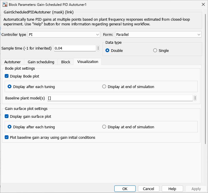
Visualization Tab
Since R2024b
Select to generate Bode plots showing the following estimated frequency response for each operating point you tune:
Plant response
Open-loop response
Reference tracking response
Controller effort response
Input disturbance rejection response
Output disturbance rejection response
You can configure the block to update the plot after tuning each breakpoint or at the end of the simulation. If you have an LTI model representing the expected plant response or other relevant baseline, include it on the plot for reference using the Baseline plant model parameter.
For an example, see Tune and Validate Gain-Scheduled PID Autotuning Results.
Since R2024b
Specify the baseline model to plot with the estimated frequency response. Use an
LTI model such as a tf, ss, or
frd model.
Example: tf(10,[1 10 1000])
Dependencies
To enable this parameter, select Display Bode plot.
Since R2024b
Select to display the plot of gain values for the each gain you tune against the scheduling variable. You can configure the block to update the plot after tuning each breakpoint or at the end of the simulation.
To plot the initial gain values before tuning, select Plot baseline gain array using gain initial conditions. You specify the base line gain values on the Gain scheduling tab.
For an example, see Tune and Validate Gain-Scheduled PID Autotuning Results.
More About
The block uses the input values to generate output using the method you select for Lookup Method:
| Lookup Method | Block Action |
|---|---|
Interpolation-Extrapolation
| Performs linear interpolation and extrapolation of the inputs.
Note If you select this lookup method, Simulink Coder™ software cannot generate code for this block. |
Interpolation-Use End Values (default) | Performs linear interpolation but does not extrapolate outside the end points of the breakpoint data. Instead, the block uses the end values. |
Use Input Nearest
| Finds the element in Breakpoints nearest the current input. The corresponding element in PID Gains is the output. |
Use Input Below
| Finds the element in Breakpoints nearest and below the current input. The corresponding element in PID Gains is the output. If there is no element in Breakpoints below the current input, the block finds the nearest element. |
Use Input Above
| Finds the element in Breakpoints nearest and above the current input. The corresponding element in PID Gains is the output. If there is no element in Breakpoints above the current input, the block finds the nearest element. |
Note
The Use Input Nearest, Use Input Below, and
Use Input Above methods perform the same action when the input
scheduling Variable matches a breakpoint value.
For more information about dynamic lookup tables, see Lookup Table Dynamic.
Extended Capabilities
C/C++ Code Generation
Generate C and C++ code using Simulink® Coder™.
Version History
Introduced in R2024aYou can now use the Gain-Scheduled PID Autotuner, PID Gain Scheduler, PID Gains Store and Update blocks to automatically tune gains with two scheduling variables. This is useful when tuning over a grid of design points defined by multiple operating conditions. To use two scheduling variables, enable Use two scheduling variables in the block parameters and specify the corresponding scheduling signals and breakpoint data.
You can now validate your gain-scheduled PID autotuning results using the new Visualization tab in the Gain-Scheduled PID Autotuner block parameters. The block allows you to visualize the frequency responses plots for the control loop, such as estimated plant, open-loop, controller effort, reference tracking, and disturbance rejection responses. The block shows responses for each operating point you tune. Additionally, you can plot the gain surface for the specified scheduling variable.
Visualizing the frequency response of the control loop is helpful when you want validate the response from the actual plant against an estimated plant. Doing so allows you to adjust the autotuning settings for a more accurate performance.
MATLAB Command
You clicked a link that corresponds to this MATLAB command:
Run the command by entering it in the MATLAB Command Window. Web browsers do not support MATLAB commands.
选择网站
选择网站以获取翻译的可用内容,以及查看当地活动和优惠。根据您的位置,我们建议您选择:。
您也可以从以下列表中选择网站:
如何获得最佳网站性能
选择中国网站(中文或英文)以获得最佳网站性能。其他 MathWorks 国家/地区网站并未针对您所在位置的访问进行优化。
美洲
- América Latina (Español)
- Canada (English)
- United States (English)
欧洲
- Belgium (English)
- Denmark (English)
- Deutschland (Deutsch)
- España (Español)
- Finland (English)
- France (Français)
- Ireland (English)
- Italia (Italiano)
- Luxembourg (English)
- Netherlands (English)
- Norway (English)
- Österreich (Deutsch)
- Portugal (English)
- Sweden (English)
- Switzerland
- United Kingdom (English)
