Build Condition Model for Industrial Machinery and Manufacturing Processes

This example builds a condition model for sensor data collected from an industrial manufacturing machine. Use the Classification Learner App to build a binary classification model that determines the condition of the machine as either "after maintenance" or "before maintenance." Train the model using the data collected both immediately before and after a scheduled maintenance. Assume that the data collected after scheduled maintenance represents normal observations, and the data collected before maintenance represents anomalies. You can use the trained model to monitor incoming observations and determine whether a new maintenance cycle is necessary by detecting anomalies in the observations.

The classification workflow in this example includes these steps:

Load data into the MATLAB^® workspace.
Import data into the Classification Learner app and reserve a percentage of the data for testing.
Train binary classification models that can detect anomalies in sensor data. Use all features in the data set.
Assess model performance using the model accuracy on the validation data.
Interrupt the app session to explore aspects of model deployment, including whether the model can fit on the target hardware within the resources designated for the classification task.
Resume the app session to build new models with reduced size. To reduce model size, train the models after selecting features using feature ranking.
Select a final model and observe its accuracy on the test set.
Export the final model for deployment on the target hardware.

Load Data

This example uses a data set that contains 12 features extracted from three-axis vibration measurements of an industrial machine. Execute the following commands to download and extract the data set file.

url = "https://ssd.mathworks.com/supportfiles/predmaint/" + ...
    "anomalyDetection3axisVibration/v1/vibrationData.zip";
outfilename = websave("vibrationData.zip",url);
unzip(outfilename)

Load the featureAll table in the FeatureEntire.mat file.

load("FeatureEntire.mat")

The table contains 17,642 observations for 13 variables (one categorical response variable and 12 predictor variables).

Shorten the predictor variable names by removing the redundant phrase ("_stats/Col1_").

for i = 2:13
    featureAll.Properties.VariableNames(i) = ...
        erase(featureAll.Properties.VariableNames(i),"_stats/Col1_");
end

Preview the first eight rows of the table.

head(featureAll)

ans=8×13 table
    label     ch1CrestFactor    ch1Kurtosis    ch1RMS    ch1Std     ch2Mean      ch2RMS     ch2Skewness    ch2Std     ch3CrestFactor    ch3SINAD    ch3SNR     ch3THD 
    ______    ______________    ___________    ______    ______    __________    _______    ___________    _______    ______________    ________    _______    _______

    Before        2.3683           1.927       2.2225    2.2225     -0.015149    0.62512      4.2931       0.62495        5.6569        -5.4476     -4.9977    -4.4608
    Before         2.402          1.9206       2.1807    2.1803     -0.018269    0.56773      3.9985       0.56744        8.7481        -12.532     -12.419    -3.2353
    Before        2.4157          1.9523       2.1789    2.1788    -0.0063652    0.45646      2.8886       0.45642        8.3111        -12.977     -12.869    -2.9591
    Before        2.4595          1.8205         2.14    2.1401     0.0017307    0.41418      2.0635       0.41418        7.2318        -13.566     -13.468    -2.7944
    Before        2.2502          1.8609       2.3391     2.339    -0.0081829     0.3694      3.3498       0.36931        6.8134         -13.33     -13.225    -2.7182
    Before        2.4211          2.2479       2.1286    2.1285      0.011139    0.36638      1.8602       0.36621        7.4712        -13.324     -13.226    -3.0313
    Before        3.3111          4.0304       1.5896    1.5896    -0.0080759    0.47218      2.1132       0.47211        8.2412         -13.85     -13.758    -2.7822
    Before        2.2655          2.0656       2.3233    2.3233    -0.0049447    0.37829      2.4936       0.37827        7.6947        -13.781     -13.683    -2.5601

The values in the first column are the labels of observations, Before or After, which indicate whether each observation is collected immediately before or after a scheduled maintenance, respectively. The remaining columns contain 12 features extracted from the vibration measurements using the Diagnostic Feature Designer app in Predictive Maintenance Toolbox™. For more information about the extracted features, see Anomaly Detection in Industrial Machinery Using Three-Axis Vibration Data (Predictive Maintenance Toolbox).

Import Data into App and Partition Data

Import the featureAll table into the Classification Learner app, and set aside 10% of the data as a test set.

On the Apps tab, click the Show more arrow to display the apps gallery. In the Machine Learning and Deep Learning group, click Classification Learner.
On the Learn tab, in the File section, click New Session > From Workspace.
In the New Session from Workspace dialog box, select the table featureAll from the Data Set Variable list. The app selects the response (label) and predictor variables (12 features) based on their data types.
In the Test section, click the check box to set aside a test data set. Specify to use 10% of the imported data as a test set. The featureAll table contains 17,642 samples, so setting aside 10% yields 1764 samples in the test set and 15,878 samples in the training set.
To accept the default validation scheme and continue, click Start Session. The default validation option is 5-fold cross-validation, to protect against overfitting.

Alternatively, you can open the Classification Learner app from the MATLAB Command Window by entering classificationLearner. You can specify the predictor data, response variable, and percentage of the data for testing.

classificationLearner(featureAll,"label",TestDataFraction=0.1)

Train Models Using All Features

First, train models using all 12 features in the data set. The Models pane already contains a draft for a fine tree model. You can add a variety of draft models to the Models pane by selecting them from the Models gallery, and then train all models.

On the Learn tab, in the Models section, click the Show more arrow to open the gallery.
Select three models:
- Bagged trees — In the Ensemble Classifiers group, click Bagged Trees.
- Fine Gaussian support vector machine (SVM) — In the Support Vector Machines group, click Fine Gaussian SVM.
- Bilayered neural network — In the Neural Network Classifiers group, click Bilayered Neural Network.
The app includes the draft models in the Models pane.
For more information on each classifier option, see Choose Classifier Options.
In the Train section of the Learn tab, click Train All and select Train All. The app trains the four models using all 12 features.
Note
- If you have Parallel Computing Toolbox™, then the Use Parallel button is selected by default. After you click Train All and select Train All or Train Selected, the app opens a parallel pool of workers. During this time, you cannot interact with the software. After the pool opens, you can continue to interact with the app while models train in parallel.
- If you do not have Parallel Computing Toolbox, then the Use Background Training check box in the Train All menu is selected by default. After you select an option to train models, the app opens a background pool. After the pool opens, you can continue to interact with the app while models train in the background.

Assess Model Performance

You can compare trained models based on multiple characteristics. For example, you can assess the model accuracy, model size (which affects memory or disk storage needs), computational costs associated with training and testing the model, and model interpretability.

Compare the four trained models based on the model accuracy measured on validation data.

In the Models pane, each model has a validation accuracy score that indicates the percentage of correctly predicted responses.

Note

Validation introduces some randomness into the results. Your model validation results can vary from the results shown in this example.

Sort the trained models based on the validation accuracy. In the Models pane, click the Sort by arrow and select Accuracy (Validation).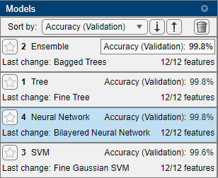
Although three of the models share the same percentage for validation accuracy, when viewed with three significant digits, the ensemble model achieves the highest accuracy by a small margin. The app highlights the ensemble model by outlining its accuracy score, and the model appears first when the models are sorted by validation accuracy.
To better understand the results, rearrange the layout of the plots so you can compare the confusion matrices for the four models. Click the Document Actions button located to the far right of the model plot tabs. Select the Tile All option and specify a 2-by-2 layout.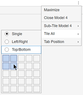
In the top right of each plot, click the Hide plot options button to make more room for the plot.
Compared to the other models, the ensemble model (Model 2) has fewer off-diagonal cells corresponding to incorrectly classified observations.

For more details on assessing model performance, see Visualize and Assess Classifier Performance in Classification Learner.

Export Model to the Workspace and Save App Session

Export the best model to the workspace and check the model size.

In the Models pane, click the ensemble model to select it.
In the Export section of the Learn tab, click Export Model and select Export Model. Exclude the training data from the exported model by clearing the check box in the Export Classification Model dialog box. You can still use the compact model for making predictions on new data.
Note
The final model exported by Classification Learner is always trained using the full data set, excluding any data reserved for testing. The validation scheme that you use only affects the way the app computes validation metrics.
In the Export Classification Model dialog box, edit the name of the exported variable, if necessary, and click OK. The default name for the exported model, trainedModel, increments every time you export (for example, trainedModel1), to avoid overwriting existing exported models.
The new variable trainedModel appears in the workspace.
Save and close the current app session. Click Save in the File section of the Learn tab. Specify the session file name and location, and then close the app.

Check Model Size

Check the exported model size by using the whos function in the Command Window.

mdl = trainedModel.ClassificationEnsemble;
whos mdl

  Name      Size             Bytes  Class                                                      Attributes

  mdl       1x1             315622  classreg.learning.classif.CompactClassificationEnsemble

Assume that you want to deploy the model on a programmable logic controller (PLC) with limited memory, and the ensemble model with all 12 features does not fit within the resources designated on the PLC.

Resume App Session

In Classification Learner, open the previously saved app session. Click Open in the File section. In the Select File to Open dialog box, select the saved session.

Select Features Using Feature Ranking

One approach to reducing model size is to reduce the number of features in a model using feature ranking and selection. Build new models with a reduced set of features and assess the model accuracy.

Create a copy of each trained model by right-clicking the model and selecting Duplicate.
To use feature ranking algorithms in Classification Learner, click Feature Selection in the Options section of the Learn tab. The app opens a Default Feature Selection tab.
In the Default Feature Selection tab, click MRMR under Feature Ranking Algorithm. The app displays a bar graph of the sorted feature importance scores, where larger scores (including Infs) indicate greater feature importance. The table on the right shows the ranked features and their scores.
Under Feature Selection, use the default option of selecting the highest ranked features to avoid bias in the validation metrics. Specify to keep 3 features for model training.
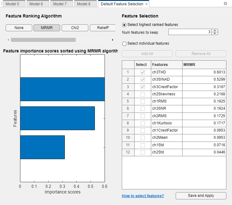
The feature ranking results are based on the full data set, including the training and validation data but not the test data. The app uses the highest ranked features to train the full model (that is, the model trained on the full data set). For each training fold, the app performs feature selection before training the model. Different folds can choose different predictors as the highest ranked features.
Click Save and Apply. The app applies the feature selection changes to the new draft models in the Models pane. Note that the draft models use 3/12 features (3 features out of 12).
In the Train section, click Train All and select Train All. The app trains all new draft models using three features.
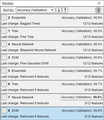
The models trained using only three features perform comparably to the models trained on all features. This result indicates that a model based on only the top three features can achieve similar accuracy as a model based on all features.
Among all the trained models, the best performing model is the neural network model with three features.

For more details on feature selection, see Feature Selection and Feature Transformation Using Classification Learner App.

Investigate Important Features in Scatter Plot

Examine the scatter plot for the best performing model using the top two features, ch3THD and ch3SINAD. The plot should show strong class separation, given the high observed model accuracies.

In the Models pane, select the best performing model (Model 7, neural network model).
On the Learn tab, in the Plots and Results section, click the Show more arrow to open the gallery, and then click Scatter in the Validation Results group.
Choose the two most important predictors, ch3THD and ch3SINAD, using the X and Y lists under Predictors.
The app creates a scatter plot of the two selected predictors, grouped by the model predictions. Because you are using cross-validation, these predictions are on the validation observations. In other words, the software obtains each prediction by using a model that was trained without the corresponding observation.
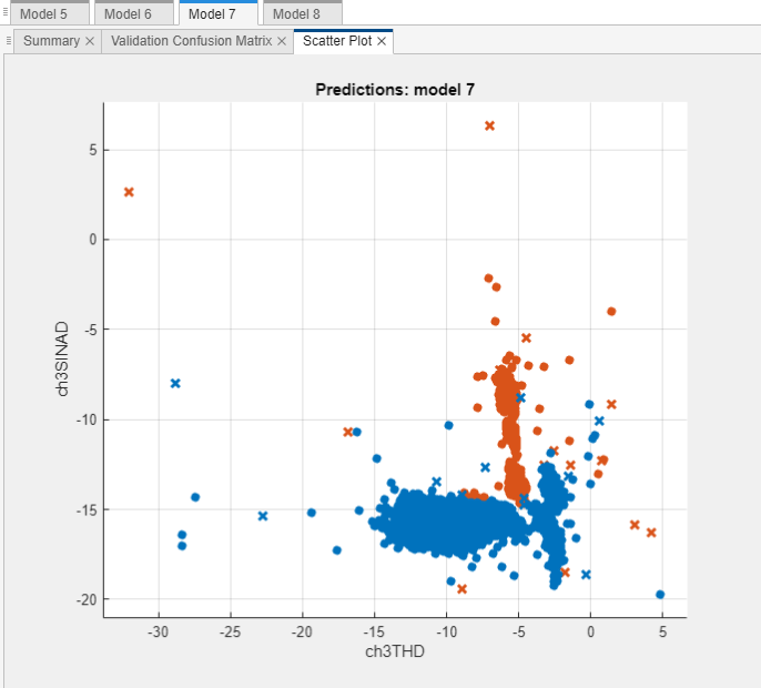
The plot shows the strong separation between the Before and After categories for the two features.

For more information, see Investigate Features in the Scatter Plot and Plot Classifier Results.

Further Experimentation

To choose a final model, you can explore further on these aspects, if necessary:

Model accuracy — To achieve better accuracy, you can explore additional model types (for example, try All in the Models gallery), further feature selection, or hyperparameter tuning. For example, before training, select a draft model in the Models pane, and then click the model Summary tab. You can specify the classifier hyperparameter options in the Model Hyperparameters section. The tab also includes Feature Selection and PCA sections with options you can set.
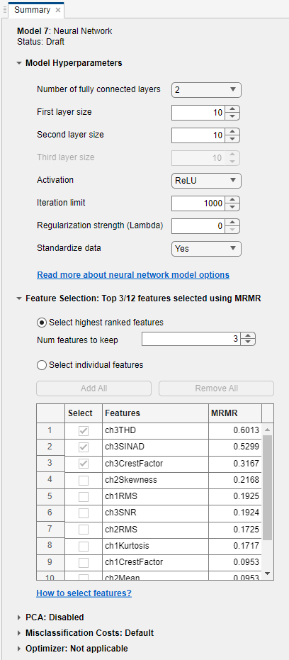
If you want to automatically tune hyperparameters of a specific model type, you can select the corresponding Optimizable model in the Models gallery and perform hyperparameter optimization. For more information, see Hyperparameter Optimization in Classification Learner App.
Computational complexity — You can find the training time and prediction speed in the Summary tab for a trained model. For example, see the Summary tab of the best performing model (Model 7, neural network model).

Assume that you decide to use the neural network model trained with the top three features based on the validation accuracy and computational complexity.

Assess Model Accuracy on Test Set

You can use the test set accuracy as an estimate of the model accuracy on unseen data. Assess the neural network model using the test set.

In the Models pane, select the neural network model.
On the Test tab, in the Test section, click Test Selected.
The app computes the test set performance of the model trained on the full data set. As expected, the model achieves similar accuracy on the test data (99.8%) compared to the validation accuracy.
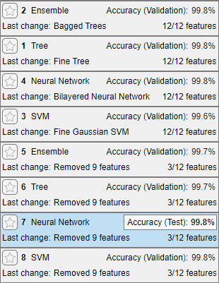
Display the confusion matrix of the test set. In the Plots and Results section on the Test tab, click Confusion Matrix (Test).

For more details, see Evaluate Test Set Model Performance.

Export Final Model

Export the final model to the workspace and check the model size.

In Classification Learner, select the neural network model in the Models pane.
In the Export section of the Learn tab, click Export Model and select Export Model.
In the Export Classification Model dialog box, edit the name of the exported variable, if necessary, and then click OK. The default name is trainedModel1.

Check the model size by using the whos function.

mdl_final = trainedModel1.ClassificationNeuralNetwork;
whos mdl_final

  Name           Size            Bytes  Class                                                           Attributes

  mdl_final      1x1              7842  classreg.learning.classif.CompactClassificationNeuralNetwork

The size of the final model (mdl_final from trainedModel1) is smaller than the size of the ensemble model (mdl from trainedModel).

For information about potential next steps of generating code for prediction or deploying predictions, see Export Classification Model to Predict New Data.