Copulas: Generate Correlated Samples

Copulas are functions that describe dependencies among variables, and provide a way to create distributions that model correlated multivariate data. Using a copula, you can construct a multivariate distribution by specifying marginal univariate distributions, and then choose a copula to provide a correlation structure between variables. Bivariate distributions, as well as distributions in higher dimensions, are possible.

Determining Dependence Between Simulation Inputs

One of the design decisions for a Monte Carlo simulation is a choice of probability distributions for the random inputs. Selecting a distribution for each individual variable is often straightforward, but deciding what dependencies should exist between the inputs may not be. Ideally, input data to a simulation should reflect what you know about dependence among the real quantities you are modeling. However, there may be little or no information on which to base any dependence in the simulation. In such cases, it is useful to experiment with different possibilities in order to determine the model's sensitivity.

It can be difficult to generate random inputs with dependence when they have distributions that are not from a standard multivariate distribution. Further, some of the standard multivariate distributions can model only limited types of dependence. It is always possible to make the inputs independent, and while that is a simple choice, it is not always sensible and can lead to the wrong conclusions.

For example, a Monte-Carlo simulation of financial risk could have two random inputs that represent different sources of insurance losses. You could model these inputs as lognormal random variables. A reasonable question to ask is how dependence between these two inputs affects the results of the simulation. Indeed, you might know from real data that the same random conditions affect both sources; ignoring that in the simulation could lead to the wrong conclusions.

Generate and Exponentiate Normal Random Variables

Open Live Script

The lognrnd function simulates independent lognormal random variables. In the following example, the mvnrnd function generates n pairs of independent normal random variables, and then exponentiates them. Notice that the covariance matrix used here is diagonal.

n = 1000;

sigma = .5;
SigmaInd = sigma.^2 .* [1 0; 0 1]

SigmaInd = 2×2

    0.2500         0
         0    0.2500

rng('default');  % For reproducibility
ZInd = mvnrnd([0 0],SigmaInd,n);
XInd = exp(ZInd);

plot(XInd(:,1),XInd(:,2),'.')
axis([0 5 0 5])
axis equal
xlabel('X1')
ylabel('X2')

Figure contains an axes object. The axes object with xlabel X1, ylabel X2 contains a line object which displays its values using only markers.

Dependent bivariate lognormal random variables are also easy to generate using a covariance matrix with nonzero off-diagonal terms.

rho = .7;
 
SigmaDep = sigma.^2 .* [1 rho; rho 1]

SigmaDep = 2×2

    0.2500    0.1750
    0.1750    0.2500

ZDep = mvnrnd([0 0],SigmaDep,n);
XDep = exp(ZDep);

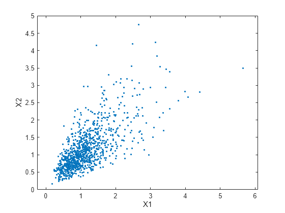
A second scatter plot demonstrates the difference between these two bivariate distributions.

plot(XDep(:,1),XDep(:,2),'.')
axis([0 5 0 5])
axis equal
xlabel('X1')
ylabel('X2')

Figure contains an axes object. The axes object with xlabel X1, ylabel X2 contains a line object which displays its values using only markers.

It is clear that there is a tendency in the second data set for large values of X1 to be associated with large values of X2, and similarly for small values. The correlation parameter $ρ$ of the underlying bivariate normal determines this dependence. The conclusions drawn from the simulation could well depend on whether you generate X1 and X2 with dependence. The bivariate lognormal distribution is a simple solution in this case; it easily generalizes to higher dimensions in cases where the marginal distributions are different lognormals.

Other multivariate distributions also exist. For example, the multivariate t and the Dirichlet distributions simulate dependent t and beta random variables, respectively. But the list of simple multivariate distributions is not long, and they only apply in cases where the marginals are all in the same family (or even the exact same distributions). This can be a serious limitation in many situations.

Constructing Dependent Bivariate Distributions

Open Live Script

Although the construction discussed in the previous section creates a bivariate lognormal that is simple, it serves to illustrate a method that is more generally applicable.

Generate pairs of values from a bivariate normal distribution. There is statistical dependence between these two variables, and each has a normal marginal distribution.
Apply a transformation (the exponential function) separately to each variable, changing the marginal distributions into lognormals. The transformed variables still have a statistical dependence.

If a suitable transformation can be found, this method can be generalized to create dependent bivariate random vectors with other marginal distributions. In fact, a general method of constructing such a transformation does exist, although it is not as simple as exponentiation alone.

By definition, applying the normal cumulative distribution function (cdf), denoted here by Φ, to a standard normal random variable results in a random variable that is uniform on the interval [0,1]. To see this, if Z has a standard normal distribution, then the cdf of U = Φ(Z) is

$\Pr {U \leq u} = \Pr {Φ (Z) \leq u} = \Pr {Z \leq Φ^{- 1} (u)} = u$

and that is the cdf of a Unif(0,1) random variable. Histograms of some simulated normal and transformed values demonstrate that fact:

n = 1000; 
rng default % for reproducibility
z = normrnd(0,1,n,1); % generate standard normal data

histogram(z,-3.75:.5:3.75,'FaceColor',[.8 .8 1]) % plot the histogram of data
xlim([-4 4])
title('1000 Simulated N(0,1) Random Values')
xlabel('Z')
ylabel('Frequency')

Figure contains an axes object. The axes object with title 1000 Simulated N(0,1) Random Values, xlabel Z, ylabel Frequency contains an object of type histogram.

u = normcdf(z);  % compute the cdf values of the sample data

figure
histogram(u,.05:.1:.95,'FaceColor',[.8 .8 1]) % plot the histogram of the cdf values
title('1000 Simulated N(0,1) Values Transformed to Unif(0,1)')
xlabel('U')
ylabel('Frequency')

Figure contains an axes object. The axes object with title 1000 Simulated N(0,1) Values Transformed to Unif(0,1), xlabel U, ylabel Frequency contains an object of type histogram.

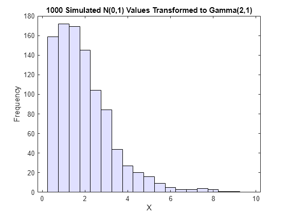
Borrowing from the theory of univariate random number generation, applying the inverse cdf of any distribution, F, to a Unif(0,1) random variable results in a random variable whose distribution is exactly F (see Inversion Methods). The proof is essentially the opposite of the preceding proof for the forward case. Another histogram illustrates the transformation to a gamma distribution:

x = gaminv(u,2,1); % transform to gamma values

figure
histogram(x,.25:.5:9.75,'FaceColor',[.8 .8 1]) % plot the histogram of gamma values
title('1000 Simulated N(0,1) Values Transformed to Gamma(2,1)')
xlabel('X')
ylabel('Frequency')

Figure contains an axes object. The axes object with title 1000 Simulated N(0,1) Values Transformed to Gamma(2,1), xlabel X, ylabel Frequency contains an object of type histogram.

You can apply this two-step transformation to each variable of a standard bivariate normal, creating dependent random variables with arbitrary marginal distributions. Because the transformation works on each component separately, the two resulting random variables need not even have the same marginal distributions. The transformation is defined as:

$\begin{array}{l} Z = [Z_{1}, Z_{2}] \sim N ([0, 0], [\begin{array}{c} 1 & ρ \\ ρ & 1 \end{array}]) \\ U = [Φ (Z_{1}), Φ (Z_{2})] \\ X = [G_{1} (U_{1}), G_{2} (U_{2})] \end{array}$

where $G_{1}$ and $G_{2}$ are inverse cdfs of two possibly different distributions. For example, the following generates random vectors from a bivariate distribution with $t_{5}$ and Gamma(2,1) marginals:

n = 1000; rho = .7;
Z = mvnrnd([0 0],[1 rho; rho 1],n);
U = normcdf(Z);
X = [gaminv(U(:,1),2,1) tinv(U(:,2),5)];

% draw the scatter plot of data with histograms 
figure
scatterhist(X(:,1),X(:,2),'Direction','out')

Figure contains 3 axes objects. Axes object 1 with xlabel x, ylabel y contains a line object which displays its values using only markers. Hidden axes object 2 contains an object of type histogram. Hidden axes object 3 contains an object of type histogram.

This plot has histograms alongside a scatter plot to show both the marginal distributions, and the dependence.

Using Rank Correlation Coefficients

Open Live Script

The correlation parameter, ρ, of the underlying bivariate normal determines the dependence between X1 and X2 in this construction. However, the linear correlation of X1 and X2 is not ρ. For example, in the original lognormal case, a closed form for that correlation is:

$cor (X1, X2) = \frac{e^{ρ σ^{2}} - 1}{e^{σ^{2}} - 1}$

which is strictly less than ρ, unless ρ is exactly 1. In more general cases such as the Gamma/t construction, the linear correlation between X1 and X2 is difficult or impossible to express in terms of ρ, but simulations show that the same effect happens.

That is because the linear correlation coefficient expresses the linear dependence between random variables, and when nonlinear transformations are applied to those random variables, linear correlation is not preserved. Instead, a rank correlation coefficient, such as Kendall's τ or Spearman's $ρ_{s}$ , is more appropriate.

Roughly speaking, these rank correlations measure the degree to which large or small values of one random variable associate with large or small values of another. However, unlike the linear correlation coefficient, they measure the association only in terms of ranks. As a consequence, the rank correlation is preserved under any monotonic transformation. In particular, the transformation method just described preserves the rank correlation. Therefore, knowing the rank correlation of the bivariate normal Z exactly determines the rank correlation of the final transformed random variables, X. While the linear correlation coefficient, ρ, is still needed to parameterize the underlying bivariate normal, Kendall's τ or Spearman's $ρ_{s}$ are more useful in describing the dependence between random variables, because they are invariant to the choice of marginal distribution.

For the bivariate normal, there is a simple one-to-one mapping between Kendall's τ or Spearman's $ρ_{s}$ , and the linear correlation coefficient ρ:

$\begin{array}{l} τ = \frac{2}{π} \arcsin (ρ) or ρ = \sin (τ \frac{π}{2}) \\ ρ_{s} = \frac{6}{π} \arcsin (\frac{ρ}{2}) or ρ = 2 \sin (ρ_{s} \frac{π}{6}) \end{array}$

The following plot shows the relationship.

rho = -1:.01:1;
tau = 2.*asin(rho)./pi;
rho_s = 6.*asin(rho./2)./pi;

plot(rho,tau,'b-','LineWidth',2)
hold on
plot(rho,rho_s,'g-','LineWidth',2)
plot([-1 1],[-1 1],'k:','LineWidth',2)
axis([-1 1 -1 1])
xlabel('rho')
ylabel('Rank correlation coefficient')
legend('Kendall''s {\it\tau}', ...
       'Spearman''s {\it\rho_s}', ... 
       'location','NW')

$Figure contains an axes object. The axes object with xlabel rho, ylabel Rank correlation coefficient contains 3 objects of type line. These objects represent Kendall's {\it\tau}, Spearman's {\it\rho_s}.$

Thus, it is easy to create the desired rank correlation between X1 and X2, regardless of their marginal distributions, by choosing the correct ρ parameter value for the linear correlation between Z1 and Z2.

For the multivariate normal distribution, Spearman's rank correlation is almost identical to the linear correlation. However, this is not true once you transform to the final random variables.

Using Bivariate Copulas

Open Live Script

The first step of the construction described in the previous section defines what is known as a bivariate Gaussian copula. A copula is a multivariate probability distribution, where each random variable has a uniform marginal distribution on the unit interval [0,1]. These variables may be completely independent, deterministically related (e.g., U2 = U1), or anything in between. Because of the possibility for dependence among variables, you can use a copula to construct a new multivariate distribution for dependent variables. By transforming each of the variables in the copula separately using the inversion method, possibly using different cdfs, the resulting distribution can have arbitrary marginal distributions. Such multivariate distributions are often useful in simulations, when you know that the different random inputs are not independent of each other.

Statistics and Machine Learning Toolbox™ functions compute:

Probability density functions (copulapdf) and the cumulative distribution functions (copulacdf) for Gaussian copulas
Rank correlations from linear correlations (copulastat) and vice versa (copulaparam)
Random vectors (copularnd)
Parameters for copulas fit to data (copulafit)

For example, use the copularnd function to create scatter plots of random values from a bivariate Gaussian copula for various levels of ρ, to illustrate the range of different dependence structures. The family of bivariate Gaussian copulas is parameterized by the linear correlation matrix:

$P = [\begin{array}{c} 1 & ρ \\ ρ & 1 \end{array}]$

U1 and U2 approach linear dependence as ρ approaches ±1, and approach complete independence as ρ approaches zero:

n = 500;

rng('default') % for reproducibility
U = copularnd('Gaussian',[1 .8; .8 1],n);
subplot(2,2,1)
plot(U(:,1),U(:,2),'.')
title('{\it\rho} = 0.8')
xlabel('U1')
ylabel('U2')

U = copularnd('Gaussian',[1 .1; .1 1],n);
subplot(2,2,2)
plot(U(:,1),U(:,2),'.')
title('{\it\rho} = 0.1')
xlabel('U1')
ylabel('U2')

U = copularnd('Gaussian',[1 -.1; -.1 1],n);
subplot(2,2,3)
plot(U(:,1),U(:,2),'.')
title('{\it\rho} = -0.1')
xlabel('U1')
ylabel('U2')

U = copularnd('Gaussian',[1 -.8; -.8 1],n);
subplot(2,2,4)
plot(U(:,1),U(:,2),'.')
title('{\it\rho} = -0.8')
xlabel('U1')
ylabel('U2')

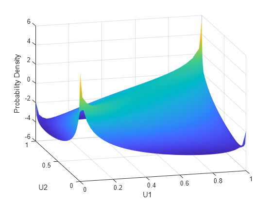
The dependence between U1 and U2 is completely separate from the marginal distributions of X1 = G(U1) and X2 = G(U2). X1 and X2 can be given any marginal distributions, and still have the same rank correlation. This is one of the main appeals of copulas—they allow this separate specification of dependence and marginal distribution. You can also compute the pdf (copulapdf) and the cdf (copulacdf) for a copula. For example, these plots show the pdf and cdf for ρ = .8:

u1 = linspace(1e-3,1-1e-3,50);
u2 = linspace(1e-3,1-1e-3,50);
[U1,U2] = meshgrid(u1,u2);
Rho = [1 .8; .8 1];
f = copulapdf('t',[U1(:) U2(:)],Rho,5);
f = reshape(f,size(U1));

figure
surf(u1,u2,log(f),'FaceColor','interp','EdgeColor','none')
view([-15,20])
xlabel('U1')
ylabel('U2')
zlabel('Probability Density')

Figure contains an axes object. The axes object with xlabel U1, ylabel U2 contains an object of type surface.

u1 = linspace(1e-3,1-1e-3,50);
u2 = linspace(1e-3,1-1e-3,50);
[U1,U2] = meshgrid(u1,u2);
F = copulacdf('t',[U1(:) U2(:)],Rho,5);
F = reshape(F,size(U1));

figure()
surf(u1,u2,F,'FaceColor','interp','EdgeColor','none')
view([-15,20])
xlabel('U1')
ylabel('U2')
zlabel('Cumulative Probability')

Figure contains an axes object. The axes object with xlabel U1, ylabel U2 contains an object of type surface.

A different family of copulas can be constructed by starting from a bivariate t distribution and transforming using the corresponding t cdf. The bivariate t distribution is parameterized with P, the linear correlation matrix, and ν, the degrees of freedom. Thus, for example, you can speak of a $t_{1}$ or a $t_{5}$ copula, based on the multivariate t with one and five degrees of freedom, respectively.

Just as for Gaussian copulas, Statistics and Machine Learning Toolbox functions for t copulas compute:

Probability density functions (copulapdf) and the cumulative distribution functions (copulacdf) for t copulas
Rank correlations from linear correlations (copulastat) and vice versa (copulaparam)
Random vectors (copularnd)
Parameters for copulas fit to data (copulafit)

For example, use the copularnd function to create scatter plots of random values from a bivariate $t_{1}$ copula for various levels of ρ, to illustrate the range of different dependence structures:

n = 500;
nu = 1;

rng('default') % for reproducibility
U = copularnd('t',[1 .8; .8 1],nu,n);
subplot(2,2,1)
plot(U(:,1),U(:,2),'.')
title('{\it\rho} = 0.8')
xlabel('U1')
ylabel('U2')

U = copularnd('t',[1 .1; .1 1],nu,n);
subplot(2,2,2)
plot(U(:,1),U(:,2),'.')
title('{\it\rho} = 0.1')
xlabel('U1')
ylabel('U2')

U = copularnd('t',[1 -.1; -.1 1],nu,n);
subplot(2,2,3)
plot(U(:,1),U(:,2),'.')
title('{\it\rho} = -0.1')
xlabel('U1')
ylabel('U2')

U = copularnd('t',[1 -.8; -.8 1],nu, n);
subplot(2,2,4)
plot(U(:,1),U(:,2),'.')
title('{\it\rho} = -0.8')
xlabel('U1')
ylabel('U2')

A t copula has uniform marginal distributions for U1 and U2, just as a Gaussian copula does. The rank correlation τ or $ρ_{s}$ between components in a t copula is also the same function of ρ as for a Gaussian. However, as these plots demonstrate, a $t_{1}$ copula differs quite a bit from a Gaussian copula, even when their components have the same rank correlation. The difference is in their dependence structure. Not surprisingly, as the degrees of freedom parameter $ν$ is made larger, a $t_{ν}$ copula approaches the corresponding Gaussian copula.

As with a Gaussian copula, any marginal distributions can be imposed over a t copula. For example, using a t copula with 1 degree of freedom, you can again generate random vectors from a bivariate distribution with Gamma(2,1) and $t_{5}$ marginals using copularnd:

n = 1000;
rho = .7;
nu = 1;

rng('default') % for reproducibility
U = copularnd('t',[1 rho; rho 1],nu,n);
X = [gaminv(U(:,1),2,1) tinv(U(:,2),5)];

figure
scatterhist(X(:,1),X(:,2),'Direction','out')

Compared to the bivariate Gamma/t distribution constructed earlier, which was based on a Gaussian copula, the distribution constructed here, based on a $t_{1}$ copula, has the same marginal distributions and the same rank correlation between variables but a very different dependence structure. This illustrates the fact that multivariate distributions are not uniquely defined by their marginal distributions, or by their correlations. The choice of a particular copula in an application may be based on actual observed data, or different copulas may be used as a way of determining the sensitivity of simulation results to the input distribution.

Higher Dimension Copulas

Open Live Script

The Gaussian and t copulas are known as elliptical copulas. It is easy to generalize elliptical copulas to a higher number of dimensions. For example, simulate data from a trivariate distribution with Gamma(2,1), Beta(2,2), and $t_{5}$ marginals using a Gaussian copula and copularnd, as follows:

n = 1000;
Rho = [1 .4 .2; .4 1 -.8; .2 -.8 1];
rng('default') % for reproducibility
U = copularnd('Gaussian',Rho,n);
X = [gaminv(U(:,1),2,1) betainv(U(:,2),2,2) tinv(U(:,3),5)];

Plot the data.

subplot(1,1,1)
plot3(X(:,1),X(:,2),X(:,3),'.')
grid on
view([-55, 15])
xlabel('X1')
ylabel('X2')
zlabel('X3')

Figure contains an axes object. The axes object with xlabel X1, ylabel X2 contains a line object which displays its values using only markers.

Notice that the relationship between the linear correlation parameter ρ and, for example, Kendall's τ, holds for each entry in the correlation matrix P used here. You can verify that the sample rank correlations of the data are approximately equal to the theoretical values:

tauTheoretical = 2.*asin(Rho)./pi

tauTheoretical = 3×3

    1.0000    0.2620    0.1282
    0.2620    1.0000   -0.5903
    0.1282   -0.5903    1.0000

tauSample = corr(X,'type','Kendall')

tauSample = 3×3

    1.0000    0.2581    0.1414
    0.2581    1.0000   -0.5790
    0.1414   -0.5790    1.0000

Archimedean Copulas

Open Live Script

Statistics and Machine Learning Toolbox™ functions are available for three bivariate Archimedean copula families:

Clayton copulas
Frank copulas
Gumbel copulas

These are one-parameter families that are defined directly in terms of their cdfs, rather than being defined constructively using a standard multivariate distribution.

To compare these three Archimedean copulas to the Gaussian and t bivariate copulas, first use the copulastat function to find the rank correlation for a Gaussian or t copula with linear correlation parameter of 0.8, and then use the copulaparam function to find the Clayton copula parameter that corresponds to that rank correlation:

tau = copulastat('Gaussian',.8 ,'type','kendall')

tau = 
0.5903

alpha = copulaparam('Clayton',tau,'type','kendall')

alpha = 
2.8820

Finally, plot a random sample from the Clayton copula with copularnd. Repeat the same procedure for the Frank and Gumbel copulas:

n = 500;

U = copularnd('Clayton',alpha,n);
subplot(3,1,1)
plot(U(:,1),U(:,2),'.');
title(['Clayton Copula, {\it\alpha} = ',sprintf('%0.2f',alpha)])
xlabel('U1')
ylabel('U2')

alpha = copulaparam('Frank',tau,'type','kendall');
U = copularnd('Frank',alpha,n);
subplot(3,1,2)
plot(U(:,1),U(:,2),'.')
title(['Frank Copula, {\it\alpha} = ',sprintf('%0.2f',alpha)])
xlabel('U1')
ylabel('U2')

alpha = copulaparam('Gumbel',tau,'type','kendall');
U = copularnd('Gumbel',alpha,n);
subplot(3,1,3)
plot(U(:,1),U(:,2),'.')
title(['Gumbel Copula, {\it\alpha} = ',sprintf('%0.2f',alpha)])
xlabel('U1')
ylabel('U2')

Simulating Dependent Multivariate Data Using Copulas

Open Live Script

To simulate dependent multivariate data using a copula, you must specify each of the following:

The copula family (and any shape parameters)
The rank correlations among variables
Marginal distributions for each variable

Suppose you have return data for two stocks and want to run a Monte Carlo simulation with inputs that follow the same distributions as the data:

load stockreturns
nobs = size(stocks,1);

subplot(2,1,1)
histogram(stocks(:,1),10,'FaceColor',[.8 .8 1])
xlim([-3.5 3.5])
xlabel('X1')
ylabel('Frequency')

subplot(2,1,2)
histogram(stocks(:,2),10,'FaceColor',[.8 .8 1])
xlim([-3.5 3.5])
xlabel('X2')
ylabel('Frequency')

Figure contains 2 axes objects. Axes object 1 with xlabel X1, ylabel Frequency contains an object of type histogram. Axes object 2 with xlabel X2, ylabel Frequency contains an object of type histogram.

You could fit a parametric model separately to each dataset, and use those estimates as the marginal distributions. However, a parametric model may not be sufficiently flexible. Instead, you can use a nonparametric model to transform to the marginal distributions. All that is needed is a way to compute the inverse cdf for the nonparametric model.

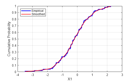
The simplest nonparametric model is the empirical cdf, as computed by the ecdf function. For a discrete marginal distribution, this is appropriate. However, for a continuous distribution, use a model that is smoother than the step function computed by ecdf. One way to do that is to estimate the empirical cdf and interpolate between the midpoints of the steps with a piecewise linear function. Another way is to use kernel smoothing with ksdensity. For example, compare the empirical cdf to a kernel smoothed cdf estimate for the first variable:

[Fi,xi] = ecdf(stocks(:,1));

figure()
stairs(xi,Fi,'b','LineWidth',2)
hold on

Fi_sm = ksdensity(stocks(:,1),xi,'function','cdf','width',.15);

plot(xi,Fi_sm,'r-','LineWidth',1.5)
xlabel('X1')
ylabel('Cumulative Probability')
legend('Empirical','Smoothed','Location','NW')
grid on

Figure contains an axes object. The axes object with xlabel X1, ylabel Cumulative Probability contains 2 objects of type stair, line. These objects represent Empirical, Smoothed.

For the simulation, experiment with different copulas and correlations. Here, you will use a bivariate t copula with a fairly small degrees of freedom parameter. For the correlation parameter, you can compute the rank correlation of the data.

nu = 5;
tau = corr(stocks(:,1),stocks(:,2),'type','kendall')

tau = 
0.5180

Find the corresponding linear correlation parameter for the t copula using copulaparam.

rho = copulaparam('t', tau, nu, 'type','kendall')

rho = 
0.7268

Next, use copularnd to generate random values from the t copula and transform using the nonparametric inverse cdfs. The ksdensity function allows you to make a kernel estimate of distribution and evaluate the inverse cdf at the copula points all in one step:

n = 1000;
U = copularnd('t',[1 rho; rho 1],nu,n);
X1 = ksdensity(stocks(:,1),U(:,1),...
               'function','icdf','width',.15);
X2 = ksdensity(stocks(:,2),U(:,2),...
               'function','icdf','width',.15);

Alternatively, when you have a large amount of data or need to simulate more than one set of values, it may be more efficient to compute the inverse cdf over a grid of values in the interval (0,1) and use interpolation to evaluate it at the copula points:

p = linspace(0.00001,0.99999,1000);
G1 = ksdensity(stocks(:,1),p,'function','icdf','width',0.15);
X1 = interp1(p,G1,U(:,1),'spline');
G2 = ksdensity(stocks(:,2),p,'function','icdf','width',0.15);
X2 = interp1(p,G2,U(:,2),'spline');

scatterhist(X1,X2,'Direction','out')

Figure contains 3 axes objects. Axes object 1 with xlabel X1, ylabel X2 contains a line object which displays its values using only markers. Hidden axes object 2 contains an object of type histogram. Hidden axes object 3 contains an object of type histogram.

The marginal histograms of the simulated data are a smoothed version of the histograms for the original data. The amount of smoothing is controlled by the bandwidth input to ksdensity.

Fitting Copulas to Data

Open Live Script

This example shows how to use copulafit to calibrate copulas with data. To generate data Xsim with a distribution "just like" (in terms of marginal distributions and correlations) the distribution of data in the matrix X, you need to fit marginal distributions to the columns of X, use appropriate cdf functions to transform X to U, so that U has values between 0 and 1, use copulafit to fit a copula to U, generate new data Usim from the copula, and use appropriate inverse cdf functions to transform Usim to Xsim.

Load and plot the simulated stock return data.

load stockreturns
x = stocks(:,1);
y = stocks(:,2);

scatterhist(x,y,'Direction','out')

Transform the data to the copula scale (unit square) using a kernel estimator of the cumulative distribution function.

u = ksdensity(x,x,'function','cdf');
v = ksdensity(y,y,'function','cdf');

scatterhist(u,v,'Direction','out')
xlabel('u')
ylabel('v')

Figure contains 3 axes objects. Axes object 1 with xlabel u, ylabel v contains a line object which displays its values using only markers. Hidden axes object 2 contains an object of type histogram. Hidden axes object 3 contains an object of type histogram.

Fit a t copula.

[Rho,nu] = copulafit('t',[u v],'Method','ApproximateML')

Rho = 2×2

    1.0000    0.7220
    0.7220    1.0000

nu = 
2.6133e+06

Generate a random sample from the t copula.

r = copularnd('t',Rho,nu,1000);
u1 = r(:,1);
v1 = r(:,2);

scatterhist(u1,v1,'Direction','out')
xlabel('u')
ylabel('v')
set(get(gca,'children'),'marker','.')

Transform the random sample back to the original scale of the data.

x1 = ksdensity(x,u1,'function','icdf'); 
y1 = ksdensity(y,v1,'function','icdf');

scatterhist(x1,y1,'Direction','out')
set(get(gca,'children'),'marker','.')

Figure contains 3 axes objects. Axes object 1 with xlabel x1, ylabel y1 contains a line object which displays its values using only markers. Hidden axes object 2 contains an object of type histogram. Hidden axes object 3 contains an object of type histogram.

As the example illustrates, copulas integrate naturally with other distribution fitting functions.