histfit
具有分布拟合的直方图
说明
示例
用均值 10 和方差 1 从正态分布生成大小为 100 的样本。
rng default; % For reproducibility
r = normrnd(10,1,100,1);
构建具有正态分布拟合的直方图。
histfit(r)
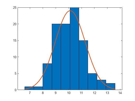
histfit 使用 fitdist 对数据进行分布拟合。使用 fitdist 获得在拟合中使用的参数。
pd = fitdist(r,'Normal')pd =
NormalDistribution
Normal distribution
mu = 10.1231 [9.89244, 10.3537]
sigma = 1.1624 [1.02059, 1.35033]
参数估计值旁边的区间是分布参数的 95% 置信区间。
用均值 10 和方差 1 从正态分布生成大小为 100 的样本。
rng default; % For reproducibility
r = normrnd(10,1,100,1);
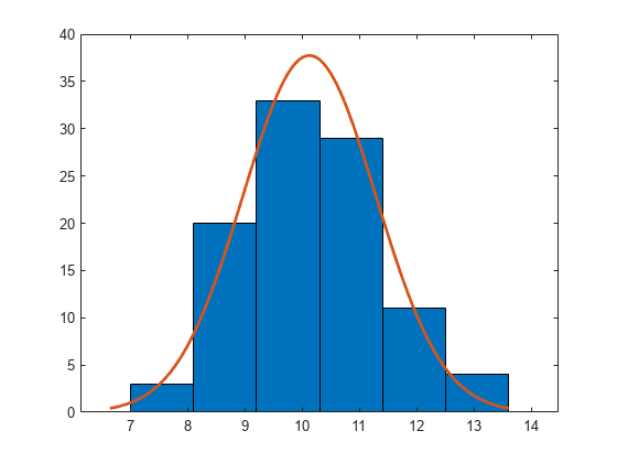
使用六个 bin 构造具有正态分布拟合的直方图。
histfit(r,6)
使用参数 (3,10) 从 beta 分布生成大小为 100 的样本。
rng default;  % For reproducibility
b = betarnd(3,10,100,1);
使用 10 个 bin 构造具有 beta 分布拟合的直方图。
histfit(b,10,'beta')
使用参数 (3,10) 从 beta 分布生成大小为 100 的样本。
rng default;  % For reproducibility
b = betarnd(3,10,[100,1]);
使用 10 个 bin 构造具有平滑函数拟合的直方图。
histfit(b,10,'kernel')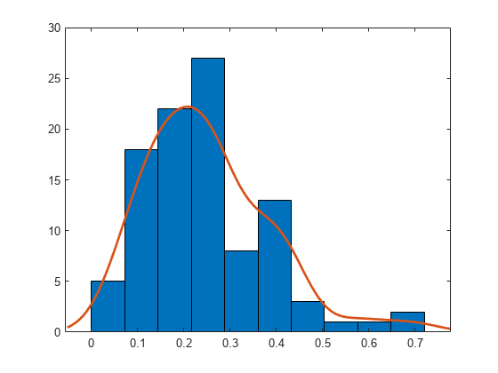
用均值 3 和方差 1 从正态分布生成大小为 100 的样本。
rng('default') % For reproducibility
r = normrnd(3,1,100,1);
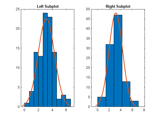
创建一个包含两个子图的图窗,并以 ax1 和 ax2 形式返回 Axes 对象。通过引用对应的 Axes 对象,在每个坐标区中创建一个具有正态分布拟合的直方图。在左侧子图中,绘制一个具有 10 个 bin 的直方图。在右侧子图中,绘制一个具有 5 个 bin 的直方图。通过将对应的 Axes 对象传递给 title 函数,为每个绘图添加标题。
ax1 = subplot(1,2,1); % Left subplot
histfit(ax1,r,10,'normal')
title(ax1,'Left Subplot')

ax2 = subplot(1,2,2); % Right subplot
histfit(ax2,r,5,'normal')
title(ax2,'Right Subplot')
用均值 10 和方差 1 从正态分布生成大小为 100 的样本。
rng default % for reproducibility
r = normrnd(10,1,100,1);
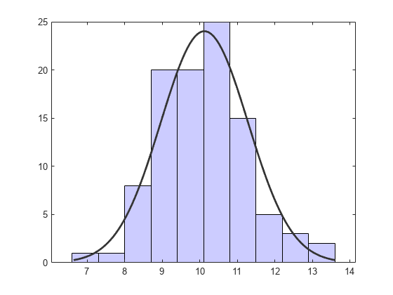
构建具有正态分布拟合的直方图。
h = histfit(r,10,'normal')
h =
  2×1 graphics array:

  Bar
  Line
更改直方图的条形颜色。
h(1).FaceColor = [.8 .8 1];

更改密度曲线的颜色。
h(2).Color = [.2 .2 .2];
输入参数
输出参量
算法
histfit 使用 fitdist 对数据进行分布拟合。使用 fitdist 获得在拟合中使用的参数。
扩展功能
版本历史记录
在 R2006a 之前推出