Stable Distribution

Overview

Stable distributions are a class of probability distributions suitable for modeling heavy tails and skewness. A linear combination of two independent, identically-distributed stable-distributed random variables has the same distribution as the individual variables. In other words, if X₁, X₂, ..., X_n are independent and identically distributed stable random variables, then for every n

$X_{1} + X_{2} + \dots + X_{n} \overset{d}{=} c_{n} X + d_{n}$

where the constant c_n > 0 and $d_{n} \in ℝ$ .

The stable distribution is an application of the Generalized Central Limit Theorem, which states that the limit of normalized sums of independent identically distributed variables is stable.

Several different parameterizations exist for the stable distribution. The implementation in Statistics and Machine Learning Toolbox™ uses the parameterization described in [2]. In this case, a random variable X has the stable distribution $S (α, β, γ, δ; 0)$ if its characteristic function is given by:

$E (e^{i t X}) = {\begin{matrix} \exp (- γ^{α} {| t |}^{α} [1 + i β sign (t) \tan \frac{π α}{2} ({(γ | t |)}^{1 - α} - 1)] + i δ t) f o r α \neq 1, \\ \exp (- γ | t | [1 + i β sign (t) \frac{2}{π} \ln (γ | t |)] + i δ t) f o r α = 1 \end{matrix}$

Parameters

The stable distribution uses the following parameters.

Parameter	Description	Support
`alpha`	First shape parameter	0 < α ≤ 2
`beta`	Second shape parameter	-1 ≤ β ≤ 1
`gam`	Scale parameter	0 < γ < ∞
`delta`	Location parameter	-∞ < δ < ∞

The first shape parameter, α, describes the tails of the distribution. The software computes the densities of the stable distribution using the direct integration method. As explained in [1], numerical difficulties exist with accurately computing the pdf and cdf when the α parameter is close to 1 or 0. If α is close to 1 (specifically, $0 < | α - 1 | < 0.02$ ), then the software rounds α to 1. If α is close to 0, then the densities may not be accurate.

The second shape parameter, β, describes the skewness of the distribution. If β = 0, then the distribution is symmetric. If β > 0, then the distribution is right-skewed. If β < 0, then the distribution is left-skewed. When α is small, the skewness of β is significant. As α increases, the effect of β decreases.

Probability Density Function

Definition

Most members of the stable distribution family do not have an explicit probability density function (pdf). Instead, the pdf is described in terms of the characteristic function [2].

Some special cases of the stable distribution, such as the normal, Cauchy, and Lévy distributions, have closed-form density functions. See Relationship to Other Distributions for more information.

Use pdf to calculate the probability density function for the stable distribution. The software computes the pdf using the direct integration method. As explained in [1], numerical difficulties exist with accurately computing the pdf when the α parameter is close to 1 or 0. If α is close to 1 (specifically, $0 < | α - 1 | < 0.02$ ), then the software rounds α to 1. If α is close to 0, then the densities may not be accurate.

Compare pdfs of Stable Distributions

Open Live Script

The following plot compares the probability density functions for stable distributions with different alpha values. In each case, beta = 0, gam = 1, and delta = 0.

pd1 = makedist('Stable','alpha',2,'beta',0,'gam',1,'delta',0);
pd2 = makedist('Stable','alpha',1,'beta',0,'gam',1,'delta',0);
pd3 = makedist('Stable','alpha',0.5,'beta',0,'gam',1,'delta',0);

Calculate the pdf for each distribution.

x = -5:.1:5;
pdf1 = pdf(pd1,x);
pdf2 = pdf(pd2,x);
pdf3 = pdf(pd3,x);

Plot all three pdf functions on the same figure for visual comparison.

figure
plot(x,pdf1,'b-');
hold on
plot(x,pdf2,'r-.');
plot(x,pdf3,'k--');
title('Compare Alpha Parameters in Stable Distribution PDF Plots')
legend('\alpha = 2','\alpha = 1','\alpha = 0.5','Location','northwest')
hold off

$Figure contains an axes object. The axes object with title Compare Alpha Parameters in Stable Distribution PDF Plots contains 3 objects of type line. These objects represent \alpha = 2, \alpha = 1, \alpha = 0.5.$

The plot illustrates the effect of the alpha parameter on the tails of the distribution.

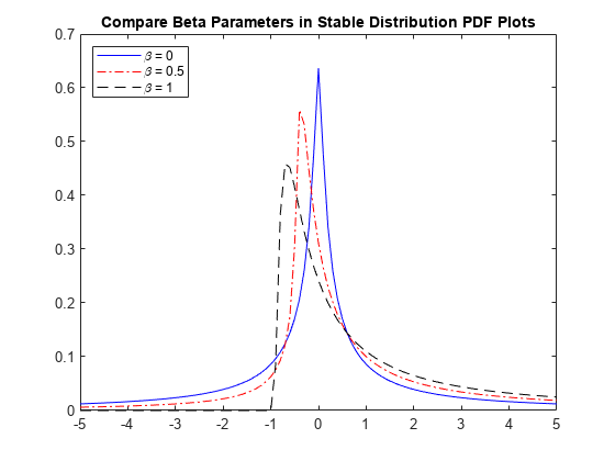
The next plot compares the probability density functions for stable distributions with different beta values. In each case, alpha = 0.5, gam = 1, and delta = 0.

pd1 = makedist('Stable','alpha',0.5,'beta',0,'gam',1,'delta',0);
pd2 = makedist('Stable','alpha',0.5,'beta',0.5,'gam',1,'delta',0);
pd3 = makedist('Stable','alpha',0.5,'beta',1,'gam',1,'delta',0);

Calculate the pdf for each distribution.

x = -5:.1:5;
pdf1 = pdf(pd1,x);
pdf2 = pdf(pd2,x);
pdf3 = pdf(pd3,x);

Plot all three pdf functions on the same figure for visual comparison.

figure
plot(x,pdf1,'b-');
hold on
plot(x,pdf2,'r-.');
plot(x,pdf3,'k--');
title('Compare Beta Parameters in Stable Distribution PDF Plots')
legend('\beta = 0','\beta = 0.5','\beta = 1','Location','northwest')
hold off

$Figure contains an axes object. The axes object with title Compare Beta Parameters in Stable Distribution PDF Plots contains 3 objects of type line. These objects represent \beta = 0, \beta = 0.5, \beta = 1.$

Random Number Generation

Use random to generate random numbers from the stable distribution. The software generates random numbers for the stable distribution using the method proposed in [3]

Cumulative Distribution Function

Definition

Most members of the stable distribution family do not have an explicit cumulative distribution function (cdf). Instead, the cdf is described in terms of the characteristic function [2].

Use cdf to calculate the cumulative distribution function for the stable distribution. The software computes the cdf using the direct integration method. As explained in [1], numerical difficulties exist with accurately computing the cdf when the α parameter is close to 1 or 0. If α is close to 1 (specifically, $0 < | α - 1 | < 0.02$ ), then the software rounds α to 1. If α is close to 0, then the densities may not be accurate.

Compare CDFs of Stable Distributions

Open Live Script

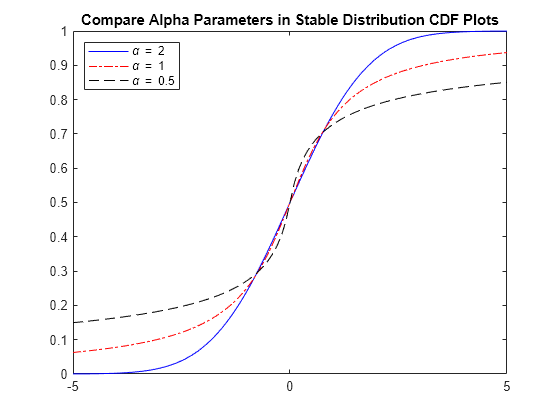
The following plot compares the cumulative distribution functions for stable distributions with different alpha values. In each case, beta = 0, gam = 1, and delta = 0.

pd1 = makedist('Stable','alpha',2,'beta',0,'gam',1,'delta',0);
pd2 = makedist('Stable','alpha',1,'beta',0,'gam',1,'delta',0);
pd3 = makedist('Stable','alpha',0.5,'beta',0,'gam',1,'delta',0);

Calculate the cdf for each distribution.

x = -5:.1:5;
cdf1 = cdf(pd1,x);
cdf2 = cdf(pd2,x);
cdf3 = cdf(pd3,x);

Plot all three cdf functions on the same figure for visual comparison.

figure
plot(x,cdf1,'b-');
hold on
plot(x,cdf2,'r-.');
plot(x,cdf3,'k--');
title('Compare Alpha Parameters in Stable Distribution CDF Plots')
legend('\alpha = 2','\alpha = 1','\alpha = 0.5','Location','northwest')
hold off

$Figure contains an axes object. The axes object with title Compare Alpha Parameters in Stable Distribution CDF Plots contains 3 objects of type line. These objects represent \alpha = 2, \alpha = 1, \alpha = 0.5.$

The plot illustrates the effect of the alpha parameter on the shape of the cdf.

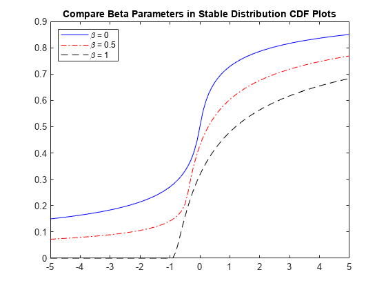
The next plot compares the cumulative distribution functions for stable distributions with different beta values. In all cases, alpha = 0.5, gam = 1, and delta = 0.

pd1 = makedist('Stable','alpha',0.5,'beta',0,'gam',1,'delta',0);
pd2 = makedist('Stable','alpha',0.5,'beta',0.5,'gam',1,'delta',0);
pd3 = makedist('Stable','alpha',0.5,'beta',1,'gam',1,'delta',0);

Calculate the cdf for each distribution.

x = -5:.1:5;
cdf1 = cdf(pd1,x);
cdf2 = cdf(pd2,x);
cdf3 = cdf(pd3,x);

Plot all three pdf functions on the same figure for visual comparison.

figure
plot(x,cdf1,'b-');
hold on
plot(x,cdf2,'r-.');
plot(x,cdf3,'k--');
title('Compare Beta Parameters in Stable Distribution CDF Plots')
legend('\beta = 0','\beta = 0.5','\beta = 1','Location','northwest')
hold off

$Figure contains an axes object. The axes object with title Compare Beta Parameters in Stable Distribution CDF Plots contains 3 objects of type line. These objects represent \beta = 0, \beta = 0.5, \beta = 1.$

Descriptive Statistics

The mean of the stable distribution is undefined for values of α ≤ 1. For α > 1, the mean of the stable distribution is

$mean = δ - β γ \tan (\frac{π α}{2}) .$

Use mean to calculate the mean of the stable distribution.

The variance of the stable distribution is undefined for values of α < 2. For α = 2, the variance of the stable distribution is

$var = 2 γ^{2} .$

Use var to calculate the variance of the stable distribution.

Relationship to Other Distributions

The stable distribution has three special cases: The normal distribution, the Cauchy distribution, and the Lévy distribution. These distributions are notable because they have closed-form probability density functions.

Normal Distribution

The normal, or Gaussian, distribution is a special case of the stable distribution. The stable distribution with α = 2 corresponds to the normal distribution. In other words,

$N (μ, σ^{2}) = S (2, 0, \frac{σ}{\sqrt{2}}, μ) .$

μ is the mean and σ is the standard deviation of the normal distribution.

Although the value of β has no effect when α = 2, the normal distribution is usually associated with β= 0.

The probability density function for the normal distribution is

$f (x) = \frac{1}{\sqrt{2 π} σ} \exp (- \frac{{(x - μ)}^{2}}{2 σ^{2}}), - \infty < x < \infty .$

A plot of the density for a normal distribution is symmetric and has a bell-shaped curve.

Cauchy Distribution

The Cauchy distribution is a special case of the stable distribution with α = 1 and β = 0. In other words,

$C a u c h y (δ, γ) = S (1, 0, γ, δ),$

where γ is the scale parameter and δ is location parameter of the Cauchy distribution.

The probability density function for the Cauchy distribution is

$f (x) = \frac{1}{π} \frac{γ}{γ^{2} + {(x - δ)}^{2}}, - \infty < x < \infty .$

A plot of the density for a Cauchy distribution is symmetric and has a bell-shaped curve, but has heavier tails than the density of a normal distribution.

Lévy Distribution

The Lévy distribution is a special case of the stable distribution where α = 0.5 and β = 1. In other words,

$L é v y (δ, γ) = S (0.5, 1, γ, γ + δ) .$

where γ is the scale parameter and δ is location parameter of the Lévy distribution.

The probability density function for the Lévy distribution is

$f (x) = \sqrt{\frac{γ}{2 π}} \frac{1}{{(x - δ)}^{3 / 2}} \exp (- \frac{γ}{2 (x - δ)}), δ < x < \infty .$

A plot of the density for a Lévy distribution is highly skewed and has heavy tails.

Comparison Plot for Stable Distributions

Open Live Script

The following plot compares the probability density functions for the standard normal, Cauchy, and Lévy distributions.

Create a probability distribution object for the standard normal, Cauchy, and Lévy distributions.

pd_norm = makedist('Stable','alpha',2,'beta',0,'gam',1/sqrt(2),'delta',0);
pd_cauchy = makedist('Stable','alpha',1,'beta',0,'gam',1,'delta',0);
pd_levy = makedist('Stable','alpha',0.5,'beta',1,'gam',1,'delta',0);

Calculate the pdf for each distribution.

x = -5:.1:5;
pdf_norm = pdf(pd_norm,x);
pdf_cauchy = pdf(pd_cauchy,x);
pdf_levy = pdf(pd_levy,x);

Plot all three pdf functions on the same figure for visual comparison.

figure
plot(x,pdf_norm,'b-');
hold on
plot(x,pdf_cauchy,'r.');
plot(x,pdf_levy,'k--');
title('Compare Stable Distributions pdf Plots')
legend('Normal','Cauchy','Levy','Location','northwest')
hold off

Figure contains an axes object. The axes object with title Compare Stable Distributions pdf Plots contains 3 objects of type line. One or more of the lines displays its values using only markers These objects represent Normal, Cauchy, Levy.

References

[1] Nolan, John P. “Numerical calculation of stable densities and distribution functions.” Communications in Statistics: Stochastic Models. Vol. 13, No. 4, 1997, pp. 759–774.

[2] Nolan, John P. Univariate Stable Distributions: Models for Heavy Tailed Data. Springer International Publishing, 2020. https://doi.org/10.1007/978-3-030-52915-4.

[3] Weron, A. and R. Weron. “Computer simulation of Lévy α-stable variables and processes.” Lecture Notes in Physics. Vol. 457, 1995, pp. 379–392.