Modulation Classification Using Wavelet Analysis on NVIDIA Jetson

Modulation Types

Specify five digital and three analog modulation types:

modTypesList = ["BPSK", ...
  "16QAM", "PAM4", "GFSK", "CPFSK", ...
  "B-FM", "DSB-AM", "SSB-AM"];
modulationTypes = categorical(modTypesList);

Specify a parent directory parentDir and the name of a directory dataDir that will be inside parentDir. You must have write permission to parentDir. The ZIP file is downloaded to parentDir. Because the example downloads data by default, dataDir must be 'wavelet_modulation_classification'. The directory dataDirectory will contain the training data used in this example. ResultDir specifies the name of a directory that will contain the trained network. ResultDir is in the same directory as this example, and will be created for you if necessary.

parentDir = tempdir;
dataDir = 'wavelet_modulation_classification';
dataDirectory = fullfile(parentDir,dataDir);
ResultDir = 'trainedNetworks';

Specify the parameters of the training data. The training data consists of 5,000 frames for each modulation type. Each frame is 1024 samples long and has a sample rate of 200 kHz. For digital modulation types, eight samples represent a symbol. Assume a center frequency of 902 MHz and 100 MHz for the digital and analog modulation types, respectively.

numFramesPerModType = 5000;
frameLength = 1024;
fs = 200e3;

Download Data

Download and unzip the training data and trained network. The dataDirectory folder contains folders named after each modulation type. The training data are in these folders. The trained network, waveletModClassNet.mat, is in ResultDir.

If you do not want to download the data, set downloadData to false. The helper function helperGenerateModWaveforms generates the frames and stores them in dataDirectory. For purposes of reproducibility, set the random seed.

downloadData = true;
if downloadData
    dataURL = 'https://ssd.mathworks.com/supportfiles/wavelet/waveletModulation/wavelet_modulation_classification.zip';
    zipFile = fullfile(parentDir,'wavelet_modulation_classification.zip');
    tic
    websave(zipFile,dataURL);
    disp(['Download time: ',num2str(toc),' seconds'])
    tic
    unzip(zipFile,parentDir);
    disp(['Unzipping time: ',num2str(toc),' seconds'])
    trainedNetworkDir = fullfile(parentDir,dataDir,'results');
    status = copyfile(trainedNetworkDir,ResultDir);
else
    rng(1235)
    helperGenerateModWaveforms(dataDirectory,modulationTypes,numFramesPerModType,frameLength,fs);
end

Download time: 38.2209 seconds

Unzipping time: 7.9005 seconds

Another example, Modulation Classification with Deep Learning (Communications Toolbox), performs modulation classification of several different modulation types using Communications Toolbox™. The helper function helperGenerateModWaveforms generates and augments a subset of the modulation types used in that example. See the example link for an in-depth description of the workflow necessary for digital and analog modulation classification and the techniques used to create these waveforms.

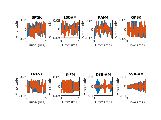
Plot the amplitude of the real and imaginary parts of a representative of each modulation type. The helper function helperModClassPlotTimeDomain2 does this.

helperModClassPlotTimeDomain2(dataDirectory,modulationTypes,fs)

Generate Scalograms

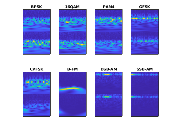
Create time-frequency representations of the waveforms. These representations are called scalograms. A scalogram is the absolute value of the CWT coefficients of a signal. To create the scalograms, precompute a CWT filter bank. Precomputing the CWT filter bank is the preferred method when obtaining the CWT of many signals using the same parameters.

Before generating all the scalograms, plot the scalograms from a representative of each modulation type. Create a CWT filter bank using cwtfilterbank for a signal with 1024 samples, and use the filter bank to take the CWT of the signal. Because the signal is complex valued, the CWT is a 3-D array. The first page is the CWT for the positive scales (analytic part or counterclockwise component), and the second page is the CWT for the negative scales (anti-analytic part or clockwise component). To generate the scalograms, take the absolute value of the concatenation of each page. The helper function helperPlotScalogramsMod2 does this.

helperPlotScalogramsMod2(dataDirectory,modulationTypes,frameLength,fs)

If you downloaded the training data and trained network, proceed to Divide into Training, Testing, and Validation Data. Otherwise, generate all the scalograms as RGB images and write them to the appropriate subdirectory in dataDirectory. The helper function helperGenerateCWTfiles2 does this. To be compatible with the SqueezeNet architecture, each RGB image is an array of size 227-by-227-by-3.

if ~downloadData
    helperGenerateCWTfiles2(dataDirectory,modulationTypes,frameLength,fs)
end

Divide into Training, Testing, and Validation Data

Load the scalogram images as an image datastore. The imageDatastore function automatically labels the images based on folder names and stores the data as an ImageDatastore object. An image datastore enables you to store large image data, including data that does not fit in memory, and efficiently read batches of images during training of a CNN.

folders = fullfile(dataDirectory,string(modulationTypes));
imds = imageDatastore(folders,...
    'FileExtensions','.jpg','LabelSource','foldernames');

Randomly divide the images into three groups, where 80% are used for training, 10% are used for validation, and 10% are used for testing. We use training and validation frames during the network training phase. For purposes of reproducibility, we set the random seed.

rng(1235)
[imdsTrain,imdsTest,imdsValidation] = splitEachLabel(imds,0.8,0.1);

If necessary, create the directory that will contain the trained network. If you downloaded the data, the directory specified by ResultDir already exists, and the file waveletModClassNet.mat in this directory contains the trained network.

if ~exist(ResultDir,'dir')
    mkdir(ResultDir)
end
MatFile = fullfile(ResultDir,'waveletModClassNet.mat');

If you downloaded the ZIP file, load the trained network and then proceed to Evaluate Network. Otherwise, you must retrain SqueezeNet.

if downloadData
    disp('Load ML model from the file')
    load(MatFile,'trainedNet','imdsValidation')
end

Load ML model from the file

SqueezeNet

SqueezeNet is a pretrained CNN that can classify images into 1000 object categories. You must retrain SqueezeNet to classify waveforms by their modulation type. Prior to retraining, you modify several network layers and set various training options. After retraining is complete, you save the CNN in a .mat file. The CUDA executable uses the .mat file.

Load SqueezeNet and extract the layer graph from the network. Inspect the last five layers of the graph.

net = squeezenet;
lgraph = layerGraph(net);
lgraph.Layers(end-4:end)

ans = 
  5×1 Layer array with layers:

     1   'conv10'                            Convolution              1000 1×1×512 convolutions with stride [1  1] and padding [0  0  0  0]
     2   'relu_conv10'                       ReLU                     ReLU
     3   'pool10'                            Global Average Pooling   Global average pooling
     4   'prob'                              Softmax                  softmax
     5   'ClassificationLayer_predictions'   Classification Output    crossentropyex with 'tench' and 999 other classes

The last learnable layer in SqueezeNet is a 1-by-1 convolutional layer, 'conv10'. Replace the layer with a new convolutional layer with the number of filters equal to the number of modulation types.

numClasses = numel(modulationTypes);
newLearnableLayer = convolution2dLayer(1,numClasses,'Name','new_conv10');
lgraph = replaceLayer(lgraph,lgraph.Layers(end-4).Name,newLearnableLayer);

Replace the classification layer with a new one without class labels. The output classes of the layer are set automatically at training time. Display the last five layers to confirm the changes.

newClassLayer = classificationLayer('Name','new_classoutput');
lgraph = replaceLayer(lgraph,lgraph.Layers(end).Name,newClassLayer);
lgraph.Layers(end-4:end)

ans = 
  5×1 Layer array with layers:

     1   'new_conv10'        Convolution              8 1×1 convolutions with stride [1  1] and padding [0  0  0  0]
     2   'relu_conv10'       ReLU                     ReLU
     3   'pool10'            Global Average Pooling   Global average pooling
     4   'prob'              Softmax                  softmax
     5   'new_classoutput'   Classification Output    crossentropyex

Train the CNN

Training a neural network is an iterative process that involves minimizing a loss function. Use the trainingOptions (Deep Learning Toolbox) function to specify options for the training process that ensures good network performance. Refer to the trainingOptions documentation for a description of each option.

OptimSolver = 'adam';
MiniBatchSize = 50;
MaxEpochs = 20;
InitialLearnRate = 1e-4;
Shuffle = 'every-epoch';

options = trainingOptions(OptimSolver, ...
    'MiniBatchSize',MiniBatchSize, ...
    'MaxEpochs',MaxEpochs, ...
    'InitialLearnRate',InitialLearnRate, ...
    'Shuffle',Shuffle, ...
    'Verbose',false, ...
    'Plots','training-progress',...
    'ValidationData',imdsValidation);

Save all the parameters in a structure. The trained network and structure will be later saved in a .mat file.

TrialParameter.OptimSolver = OptimSolver;
TrialParameter.MiniBatchSize = MiniBatchSize;
TrialParameter.MaxEpochs = MaxEpochs;
TrialParameter.InitialLearnRate = InitialLearnRate;

Set the random seed to the default value and use the trainNetwork (Deep Learning Toolbox) function to train the CNN. Save the trained network, trial parameters, training run time, and image datastore containing the validation images. Because of the dataset's large size, the process will take many minutes. By default, training is done on a GPU if one is available. Using a GPU requires Parallel Computing Toolbox™. To see which GPUs are supported, see GPU Computing Requirements (Parallel Computing Toolbox). Otherwise, training is done on the CPU. The training accuracy plots in the figure show the progress of the network's learning across all iterations.

if ~downloadData
    rng default
    tic;
    trainedNet = trainNetwork(imdsTrain,lgraph,options);
    trainingTime = toc;
    fprintf('Total training time: %.2e sec\n',trainingTime);
    save(MatFile,'TrialParameter','trainedNet','trainingTime','imdsValidation');
end

Evaluate Network

Load the .mat file that contains the trained network and the training parameters. Save only the trained network in a separate .mat file. This file will be used by the CUDA executable.

OutMatFile = 'mdwv_model.mat';
data = load(MatFile,'trainedNet');
trainedNet = data.trainedNet;
save(OutMatFile,'trainedNet');

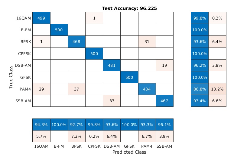
Evaluate the trained network by obtaining the classification accuracy for the test frames.

[YPred,probs] = classify(trainedNet,imdsTest);
imdsTestLabels = imdsTest.Labels;
modAccuracy = sum(YPred==imdsTestLabels)/numel(imdsTestLabels)*100

modAccuracy = 96.2250

Summarize the performance of the trained network on the test frames with a confusion chart. Display the precision and recall for each class by using column and row summaries. Save the figure. The table at the bottom of the confusion chart shows the precision values. The table to the right of the confusion chart shows the recall values.

figure('Units','normalized','Position',[0.2 0.2 0.5 0.5]);
ccDCNN = confusionchart(imdsTestLabels,YPred);
ccDCNN.Title = ['Test Accuracy: ',num2str(modAccuracy)];
ccDCNN.ColumnSummary = 'column-normalized';
ccDCNN.RowSummary = 'row-normalized';
AccFigFile = fullfile(ResultDir,'Network_ValidationAccuracy.fig');
saveas(gcf,AccFigFile);

Display the size of the trained network.

info = whos('trainedNet');
ModelMemSize = info.bytes/1024;
fprintf('Trained network size: %g kB\n',ModelMemSize)

Trained network size: 2992.95 kB

Determine the average time it takes the network to classify an image.

NumTestForPredTime = 20;
TrialParameter.NumTestForPredTime = NumTestForPredTime;

fprintf('Test prediction time (number of tests: %d)... ',NumTestForPredTime)

Test prediction time (number of tests: 20)... 

imageSize = trainedNet.Layers(1).InputSize;
PredTime = zeros(NumTestForPredTime,1);
for i = 1:NumTestForPredTime
    x = randn(imageSize);
    tic;
    [YPred, probs] = classify(trainedNet,x);
    PredTime(i) = toc;
end
AvgPredTimePerImage = mean(PredTime);
fprintf('Average prediction time: %.2e sec \n',AvgPredTimePerImage);

Average prediction time: 8.41e-02 sec 

Save the results.

if ~downloadData
    save(MatFile,'modAccuracy','ccDCNN','PredTime','ModelMemSize', ...
        'AvgPredTimePerImage','-append')
end

GPU Code Generation — Define Functions

The scalogram of a signal is the input "image" to a deep CNN. Create a function, cwtModType, that computes the scalogram of the complex-valued waveform and returns an image at the user-specified dimensions. The image uses the jet(128) colormap. For purposes of code generation, treat the input signal as a 1024-by-2 matrix, where the first column contains the real parts of the waveform samples, and the second column contains the imaginary parts. The %#codegen directive in the function indicates that the function is intended for code generation. When using the coder.gpu.kernelfun pragma, code generation attempts to map the computations in the cwtModType function to the GPU.

type cwtModType

function im = cwtModType(inputSig, imgSize)  %#codegen
% This function is only intended to support wavelet deep learning examples.
% It may change or be removed in a future release.
coder.gpu.kernel;

% Input is a 1024x2 matrix, convert it into complex form (a + 1*ib)
cinputSig = convertToComplex(inputSig);

% Wavelet time-frequency representations
[wt, ~, ~] = cwt(cinputSig, 'morse', 1, 'VoicesPerOctave', 48);

% Generate Wavelet Time-Frequency Coefficients from Signal
cfs = abs([wt(:,:,1); wt(:,:,2)]); % Concatenate the clockwise and counterclockwise representation

% Image generation
im = generateImagefromCWTCoeff(cfs, imgSize);
end

Create the entry-point function, modelPredictModType, for code generation. The function takes complex-valued signal, specified as a 1024-by-2 matrix, as input and calls the cwtModType function to create an image of the scalogram. The modelPredictModType function uses the network contained in the mdwv_model file to classify the waveform.

type modelPredictModType

function predClassProb = modelPredictModType(inputSig) %#codegen
% This function is only intended to support wavelet deep learning examples.
% It may change or be removed in a future release.
coder.gpu.kernelfun();
% input signal size is 1024-by-2

% parameters
ModelFile = 'mdwv_model.mat'; % file that saves the neural network model
imSize = [227 227]; % Size of the input image for the deep learning network

%Function to converts signal to wavelet time-frequency image
im = cwtModType(inputSig, imSize);

%Load the trained deep learning network
persistent model;
if isempty(model)
    model = coder.loadDeepLearningNetwork(ModelFile, 'mynet');
end

% Predict the Signal Modulation
predClassProb = model.predict(im);
end

To generate a CUDA executable that can be deployed to an NVIDIA target, create a custom main file (main_mod_jetson.cu) and a header file (main_mod_jetson.h). You can generate an example main file and use that as a template to rewrite new main and header files. For more information, see the GenerateExampleMain property of coder.CodeConfig (MATLAB Coder). The main file calls the code generated for the MATLAB entry-point function. The main file first reads the waveform signal from a text file, passes the data to the entry-point function, and writes the prediction results to a text file (predClassProb.txt). To maximize computation efficiency on the GPU, the executable processes single-precision data.

If you want to view the contents of the main and header files, set viewFiles to true.

viewFiles = false;
if viewFiles
    type main_mod_jetson.cu
end
if viewFiles
    type main_mod_jetson.h
end

GPU Code Generation — Connect to Hardware

To communicate with the NVIDIA hardware, you create a live hardware connection object using the jetson function. You must know the host name or IP address, user name, and password of the target board to create a live hardware connection object.

Create a live hardware connection object for the Jetson hardware. In the following code, replace:

During the creation of the object, the software performs hardware and software checks, IO server installation, and gathers information on the peripherals connected to the target. This information is displayed in the command window.

hwobj = jetson("NameOfJetsonDevice","Username","password");

Checking for CUDA availability on the Target...
Checking for 'nvcc' in the target system path...
Checking for cuDNN library availability on the Target...
Checking for TensorRT library availability on the Target...
Checking for prerequisite libraries is complete.
Gathering hardware details...
Checking for third-party library availability on the Target...
Gathering hardware details is complete.
 Board name         : NVIDIA Jetson TX1, NVIDIA Jetson Nano
 CUDA Version       : 10.0
 cuDNN Version      : 7.3
 TensorRT Version   : 5.0
 GStreamer Version  : 1.14.5
 V4L2 Version       : 1.14.2-1
 SDL Version        : 1.2
 Available Webcams  :  
 Available GPUs     : NVIDIA Tegra X1

Use the coder.checkGpuInstall (GPU Coder) function and verify that the compilers and libraries needed for running this example are set up correctly on the hardware.

envCfg = coder.gpuEnvConfig('jetson');
envCfg.DeepLibTarget = 'cudnn';
envCfg.DeepCodegen = 1;
envCfg.HardwareObject = hwobj;
envCfg.Quiet = 1;
coder.checkGpuInstall(envCfg)

ans = struct with fields:
                 gpu: 1
                cuda: 1
               cudnn: 1
            tensorrt: 0
        basiccodegen: 0
       basiccodeexec: 0
         deepcodegen: 1
        deepcodeexec: 0
    tensorrtdatatype: 0
           profiling: 0

GPU Code Generation — Specify Target

To create an executable that can be deployed to the target device, set CodeGenMode equal to 1. If you want to create an executable that runs locally and connects remotely to the target device, set CodeGenMode equal to 2. Jetson_BuildDir specifies the directory for performing the remote build process on the target. If the specified build directory does not exist on the target, then the software creates a directory with the given name.

CodeGenMode = 1;
Function_to_Gen = 'modelPredictModType';
ModFile = 'mdwv_model.mat'; % file that saves neural network model; consistent with "main_mod_jetson.cu"
ImgSize = [227 227]; % input image size for the ML model
Jetson_BuildDir = '~/projectMDWV';

Create a GPU code configuration object necessary for compilation. Use the coder.hardware function to create a configuration object for the Jetson platform and assign it to the Hardware property of the code configuration object cfg. Use 'NVIDIA Jetson' for the Jetson TX1 or TX2 boards. The custom main file is a wrapper that calls the entry-point function in the generated code. The custom file is required for a deployed executable.

Use the coder.DeepLearningConfig (GPU Coder) function to create a CuDNN deep learning configuration object and assign it to the DeepLearningConfig property of the GPU code configuration object. The code generator takes advantage of NVIDIA® CUDA® deep neural network library (cuDNN) for NVIDIA GPUs. cuDNN is a GPU-accelerated library of primitives for deep neural networks.

if CodeGenMode == 1
    cfg = coder.gpuConfig('exe');
    cfg.Hardware = coder.hardware('NVIDIA Jetson');
    cfg.Hardware.BuildDir = Jetson_BuildDir;
    cfg.DeepLearningConfig = coder.DeepLearningConfig('cudnn');
    cfg.CustomSource = 'main_mod_jetson.cu';
elseif CodeGenMode == 2
    cfg = coder.gpuConfig('lib');
    cfg.VerificationMode = 'PIL';
    cfg.Hardware = coder.hardware('NVIDIA Jetson');
    cfg.Hardware.BuildDir = Jetson_BuildDir;
    cfg.DeepLearningConfig = coder.DeepLearningConfig('cudnn');
end

GPU Code Generation — Compile

To generate CUDA code, use the codegen function and pass the GPU code configuration along with the size and type of the input for the modelPredictModType entry-point function. After code generation on the host is complete, the generated files are copied over and built on the target.

codegen('-config ',cfg,Function_to_Gen,'-args',{single(ones(1024,2))},'-report');

Code generation successful: View report

GPU Code Generation — Choose Signal

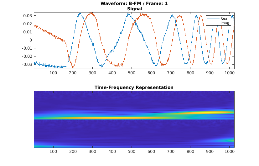
The CUDA executable performs modulation classification by generating the scalogram of the complex-valued waveform and applying the retrained CNN to the scalogram. Choose a waveform that was generated at the beginning of this example. From the 5,000 frames of each modulation type, select one of the first 50 frames generated by setting waveNumber. Plot the real and imaginary parts of the frame, and the scalogram generated from it. Use the helper function helperPlotWaveFormAndScalogram. You can find the source code for this helper function in the Supporting Functions section at the end of this example.

waveForm = modTypesList(6);
waveNumber =  1;
signal_data = helperPlotWaveFormAndScalogram(dataDirectory,waveForm,waveNumber);

If you compiled an executable to be deployed to the target, write the signal you chose to the text file signalFile. Use the putFile() function of the hardware object to place the text file on the target. The workspaceDir property contains the path to the codegen folder on the target. The main function in the executable reads data from the text file specified by signalFile and writes the classification results to resultFile.

signalFile = 'signalData.txt';
resultFile = 'predClassProb.txt'; % consistent with "main_mod_jetson.cu"

if CodeGenMode == 1
    fid = fopen(signalFile,'w');
    for i = 1:length(signal_data)
        fprintf(fid,'%f\n',real(signal_data(i)));
    end
    for i = 1:length(signal_data)
        fprintf(fid,'%f\n',imag(signal_data(i)));
    end
    fclose(fid);
    hwobj.putFile(signalFile,hwobj.workspaceDir);
end

GPU Code Generation — Execute

Run the executable.

When running the deployed executable, delete the previous result file if it exists. Use the runApplication() function to launch the executable on the target hardware, and then the getFile() function to retrieve the results. Because the results may not exist immediately after the runApplication() function call returns, and to allow for communication delays, set a maximum time for fetching the results to 90 seconds. Use the evalc function to suppress the command-line output.

if CodeGenMode == 1 % run deployed executable
    maxFetchTime = 90;
    resultFile_hw = fullfile(hwobj.workspaceDir,resultFile);
    if ispc
        resultFile_hw = strrep(resultFile_hw,'\','/');
    end
    
    ta = tic;
    
    hwobj.deleteFile(resultFile_hw)
    evalc('hwobj.runApplication(Function_to_Gen,signalFile)');
    
    tf = tic;
    success = false;
    while toc(tf) < maxFetchTime
        try
            evalc('hwobj.getFile(resultFile_hw)');
            success = true;
        catch ME
        end
        if success
            break
        end
    end
    fprintf('Fetch time = %.3e sec\n',toc(tf));
    assert(success,'Unable to fetch the prediction')
    PredClassProb = readmatrix(resultFile);
    PredTime = toc(ta);
elseif CodeGenMode == 2 % run PIL executable
    sigData = [real(signal_data)';imag(signal_data)']';
    ta = tic;
    eval(sprintf('PredClassProb = %s_pil(single(sigData));',Function_to_Gen));
    PredTime = toc(ta);
    eval(sprintf('clear %s_pil;',Function_to_Gen)); % terminate PIL execution
end

Fetch time = 4.852e+00 sec

GPU Code Generation — Display Result

The resultFile contains the classification results. For each possible modulation type, the network assigned a probability that the signal was of that type. Display the chosen modulation type. Use the helper function helperPredViz to display the classification results.

if CodeGenMode == 1
    helperPredViz                   % read fetched prediction results file
elseif CodeGenMode == 2
    helperPredVizPil(PredClassProb) % read workspace variable
end

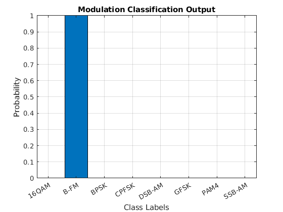
fprintf('Expected Waveform: %s\n',waveForm);

Expected Waveform: B-FM

Summary

This example shows how to create and deploy a CUDA executable that uses a CNN to perform modulation classification. You also have the option to create an executable the runs locally and connects to the remote target. A complete workflow is presented in this example. After the data is downloaded, the CWT is used to extract features from the waveforms. Then SqueezeNet is retrained to classify the signals based on their scalograms. Two user-defined functions are created and compiled on the target NVIDIA device. Results of the executable are compared with MATLAB.

Supporting Functions

helperPlotWaveFormAndScalogram

function sig = helperPlotWaveFormAndScalogram(dataDirectory,wvType,wvNum)
% This function is only intended to support wavelet deep learning examples.
% It may change or be removed in a future release.

waveFileName = sprintf('frame%s%05d.mat',wvType,wvNum);
load(fullfile(dataDirectory,wvType,waveFileName),'frame');
sig = frame;

cfs = cwt(sig,'morse',1,'VoicesPerOctave',48);
cfs = abs([cfs(:,:,1);cfs(:,:,2)]);

subplot(211)
plot(real(frame))
hold on
plot(imag(frame))
hold off
axis tight
legend('Real','Imag')
str = sprintf('Waveform: %s / Frame: %d\n Signal',wvType,wvNum);
title(str)

subplot(212)
imagesc(cfs)
title('Time-Frequency Representation')
%set(gca,'xtick',[]);
set(gca,'ytick',[]);

end

helperPredVizPil

function helperPredVizPil(PredClassProb)
% This function is only intended to support wavelet deep learning examples.
% It may change or be removed in a future release.

classNames = {'16QAM';'B-FM';'BPSK';'CPFSK';'DSB-AM';'GFSK';'PAM4';'SSB-AM'};
figure
bar(PredClassProb)
set(gca, 'XTickLabel' , classNames)
xlabel('Class Labels')
ylabel('Probability')
title('Modulation Classification Output')
axis tight
grid on

end