Block Codes
Block-Coding Features
Error-control coding techniques detect, and possibly correct, errors that occur when messages are transmitted in a digital communications system. To accomplish this, the encoder transmits not only the information symbols but also extra redundant symbols. The decoder interprets the received signal, using the redundant symbols to detect and possibly correct errors that occurred during transmission. You might use error-control coding if your transmission channel is very noisy or if your data is very sensitive to noise. Depending on the nature of the data or noise, you might choose a specific type of error-control coding.
Block coding is a special case of error-control coding that treats each block of data independently and uses a memoryless coder device. Block-coding techniques map a fixed number of message symbols to a fixed number of code symbols. Communications Toolbox™ contains MATLAB® functions and System objects, and Simulink® blocks that provide block-coding capabilities. The block-coding techniques include categories shown in this diagram.
Features in Communications Toolbox can encode and decode a message by using general linear block codes — including low-density parity-check (LDPC), cyclic, Bose–Chaudhuri–Hocquenghem (BCH), Hamming, and Reed-Solomon codes (which are all special kinds of linear block codes). The Reed-Solomon and BCH decoders indicate how many errors they detected while decoding. The Reed-Solomon coding blocks also let you decide whether to use symbols or bits as your data. Use these features to generate various linear block codes.
| Functions | System objects | Blocks | |
|---|---|---|---|
| Linear Block Codes | — | Binary Cyclic Encoder, Binary Cyclic Decoder | |
| BCH Codes | |||
| Turbo Product Codes | — | ||
| Hamming Codes | — | ||
| Reed-Solomon Codes | Binary-Input RS Encoder, Binary-Output RS Decoder Integer-Input RS Encoder, Integer-Output RS Decoder Integer-Input RS Encoder HDL Optimized, Integer-Output RS Decoder HDL Optimized | ||
| LDPC Codes | — |
Terminology
Throughout this section, the information to be encoded consists of message symbols and the code that is produced consists of codewords.
K or k represent the message length, N or n represent the codeword length, and the code is called an [N,K] code. Each block of K message symbols is encoded into a codeword that consists of N coded message symbols.
Data Formats for Block Coding
Each message or codeword is an ordered grouping of symbols. Each block in the Block Coding sublibrary processes one word in each time step, as described in the following section, Binary Format (All Coding Methods). Reed-Solomon coding blocks also let you choose between binary and integer data, as described in Integer Format (Reed-Solomon Only).
Binary Format (All Coding Methods)
You can structure messages and codewords as binary vector signals, where each vector represents a message word or a codeword. At a given time, the encoder receives an entire message word, encodes it, and outputs the entire codeword. The message and code signals operate over the same sample time.
This example illustrates the encoder receiving a four-bit message and producing a five-bit codeword at time 0. It repeats this process with a new message at time 1.
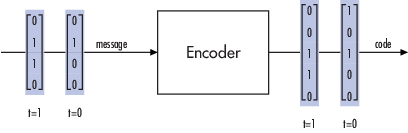
For the coding techniques, the message vector must have length K and the corresponding code vector has length N.
Note
For Reed-Solomon codes with binary input, the symbols for the code are binary sequences of length M, corresponding to elements of the Galois field GF(2M). In this case, the message vector must have length (M×K) and the corresponding code vector has length (M×K). The Binary-Input RS Encoder and Binary-Output RS Decoder blocks use this format for messages and codewords.
If the input to a block-coding block is a frame-based vector, it must be a column vector instead of a row vector.
To produce sample-based messages in the binary format, you can configure the Bernoulli Binary Generator block so that its Probability of a zero parameter is a vector whose length is that of the signal you want to create. To produce frame-based messages in the binary format, you can configure the same block so that its Probability of a zero parameter is a scalar and its Samples per frame parameter is the length of the signal you want to create.
Using Serial Signals
If you prefer to structure messages and codewords as scalar signals, where several samples jointly form a message word or codeword, you can use the Buffer and Unbuffer blocks. Buffering involves latency and multirate processing. If your model computes error rates, the initial delay in the coding-buffering combination influences the Receive delay parameter in the Error Rate Calculation block.
You can display the sample times of signals in your model. On the Debug tab, expand Information Overlays. In the Sample Time section, select Colors. Alternatively, you can attach Probe (Simulink) blocks to connector lines to help evaluate sample timing, buffering, and delays.
Integer Format (Reed-Solomon Only)
A message word for an [N,K] Reed-Solomon code consists of M×K bits, which you can interpret as K symbols from 0 to 2M. The symbols are binary sequences of length M, corresponding to elements of the Galois field GF(2M), in descending order of powers. The integer format for Reed-Solomon codes lets you structure messages and codewords as integer signals instead of binary signals. (The input must be a frame-based column vector.)
Note
In this context, Simulink expects the first bit to be the most significant bit in the symbol, as well as the smallest index in a vector or the smallest time for a series of scalars.
This figure illustrates the equivalence between binary and integer signals for a Reed-Solomon encoder. The case for the decoder is similar.
![This image shows integer versus binary formatting of data input to the RS encoder. The diagram compares two input formats for Reed-Solomon (RS) encoding. On the left, a vertical vector of 15 binary bits (0s and 1s) is grouped in two ways: the top shows grouping into 5 symbols of 3 bits each, forming a vector [3, 7, 0, 1, 1], which is input to the "RS encoder" (labeled "Integer format versus Binary format"). The bottom shows the original 15-bit vector as a "Vector of 3 x 5 bits" input directly to a "Binary Input RS encoder." Arrows indicate the flow of data to each encoder.](integerformat.png)
To produce sample-based messages in the integer format, you can configure the Random Integer Generator block so that M-ary number and Initial seed parameters are vectors of the desired length and all entries of the M-ary number vector are 2M. To produce frame-based messages in the integer format, you can configure the same block so that its M-ary number and Initial seed parameters are scalars and its Samples per frame parameter is the length of the signal you want to create.
Using Block Encoders and Decoders Within a Model
Once you have configured the coding blocks, a few tips can help you place them correctly within your model:
If a block has multiple outputs, the first one is always the stream of coding data. The Reed-Solomon and BCH blocks have an error counter as a second output.
Be sure that the signal sizes are appropriate for the mask parameters. For example, if you use the Binary Cyclic Encoder block and set Message length K to
4, the input signal must be a vector of length 4.You can display the size of signals in your model. On the Debug tab, expand Information Overlays, and then in the Signals section, select Signal Dimensions.
Notes on Specific Block-Coding Techniques
Although the Block Coding sublibrary is somewhat uniform in its look and feel, the various coding techniques are not identical. This section describes special options and restrictions that apply to parameters and signals for the coding technique categories in this sublibrary. Coding techniques discussed below include - Generic Linear Block code, Cyclic code, Hamming code, BCH code, and Reed-Solomon code.
Generic Linear Block Codes
Encoding a message using a generic linear block code requires a generator matrix. Decoding the code requires the generator matrix and possibly a truth table. To use the Binary Linear Encoder and Binary Linear Decoder blocks, you must understand the Generator matrix and Error-correction truth table parameters.
Generator Matrix - The process of encoding a message into an [N,K] linear block code is determined by a K-by-N generator matrix G. Specifically, a 1-by-K message vector v is encoded into the 1-by-N codeword vector vG. If G has the form [Ik, P] or [P, Ik], where P is some K-by-(N-K) matrix and Ik is the K-by-K identity matrix, G is said to be in standard form. (Some authors, such as Clark and Cain [2], use the first standard form, while others, such as Lin and Costello [3], use the second.) The linear block-coding blocks in this product require the Generator matrix mask parameter to be in standard form.
Decoding Table - A decoding table tells a decoder how to correct errors that may have corrupted the code during transmission. Hamming codes can correct any single-symbol error in any codeword. Other codes can correct, or partially correct, errors that corrupt more than one symbol in a given codeword.
The Binary Linear Decoder block allows you to specify a decoding table in the Error-correction truth table parameter. Represent a decoding table as a matrix with N columns and 2N-K rows. Each row gives a correction vector for one received codeword vector.
You can avoid specifying a decoding table explicitly, by setting the
Error-correction truth table parameter to
0. When Error-correction truth table is
0, the block computes a decoding table using the syndtable function.
Cyclic Codes
For cyclic codes, the codeword length N must have the form 2M–1, where M is an integer greater than or equal to 3.
Generator Polynomials - Cyclic codes have special algebraic properties that allow a polynomial to determine the coding process completely. This so-called generator polynomial is a degree-(N–K) divisor of the polynomial xN–1. Van Lint [5] explains how a generator polynomial determines a cyclic code.
The Binary Cyclic Encoder and Binary Cyclic Decoder blocks allow you to specify a generator
polynomial as the second mask parameter, instead of specifying K
there. The blocks represent a generator polynomial using a vector that lists the
coefficients of the polynomial in order of ascending powers of
the variable. You can find generator polynomials for cyclic codes using the
cyclpoly function.
If you do not want to specify a generator polynomial, set the second mask parameter to the value of K.
Hamming Codes
For Hamming codes, the codeword length N must have the form 2M–1, where M is an integer greater than or equal to 3. The message length K must equal N–M.
Primitive Polynomials - Hamming codes rely on algebraic
fields that have 2M elements (or, more
generally, pM
elements for a prime number p). Elements of such fields are named
relative to a distinguished element of the field that is
called a primitive element. The minimal polynomial of a
primitive element is called a primitive polynomial. The Hamming Encoder and Hamming Decoder blocks allow you to specify a primitive polynomial for
the finite field that they use for computations. If you want to specify this
polynomial, do so in the second mask parameter field. The blocks represent a
primitive polynomial using a vector that lists the coefficients of the polynomial in
order of ascending powers of the variable. You can find
generator polynomials for Galois fields using the gfprimfd function.
If you do not want to specify a primitive polynomial, set the second mask parameter to the value of K.
BCH Codes
BCH codes are cyclic error-correcting codes that are constructed using finite
fields. For these codes, the codeword length N must have the form
2M–1, where
M is an integer from 3 to 9. The message length
K is restricted to particular values that depend on N. To see
which values of K are valid for a given N, see
the comm.BCHEncoder
System object™ reference page. No known analytic formula describes the relationship
among the codeword length, message length, and error-correction capability for BCH
codes.
Narrow-Sense BCH Codes
The narrow-sense generator polynomial is LCM[m_1(x), m_2(x), ..., m_2t(x)], where:
LCM represents the least common multiple,
m_i(x) represents the minimum polynomial corresponding to αi, α is a root of the default primitive polynomial for the field GF(n+1),
and t represents the error-correcting capability of the code.
Reed-Solomon Codes
Reed-Solomon codes are useful for correcting errors that occur in bursts. In the
simplest case, the length of codewords in a Reed-Solomon code is of the form N= 2M – 1, where the 2M is the
number of symbols for the code. The error-correction capability of a Reed-Solomon
code is floor((N–K)/2), where K is the length
of message words. The difference (N–K) must be even.
It is sometimes convenient to use a shortened Reed-Solomon code in which
N is less than 2M–1. In this case, the encoder appends 2M–1–N zero symbols to each message word and codeword. The
error-correction capability of a shortened Reed-Solomon code is also
floor((N-K)/2). Reed-Solomon blocks and System objects in
Communications Toolbox software can implement shortened Reed-Solomon codes.
Effect of Nonbinary Symbols — Reed-Solomon codes process symbols in GF(2M), where M bits specify each symbol. The other codes supported in Communications Toolbox software process symbols in GF(2). The nonbinary nature of the Reed-Solomon code symbols causes Reed-Solomon coding to differ from other coding in these ways:
You can use the integer format, with the blocks (Integer-Input RS Encoder and Integer-Output RS Decoder) and System objects (
comm.RSEncoderandcomm.RSDecoder).The binary format expects the vector lengths to be an integer multiple of (M×K), instead of K, for messages and (M×N), instead of N, for codewords.
Error Information — The Reed-Solomon decoding blocks (Binary-Output RS Decoder and Integer-Output RS Decoder) and System object (comm.RSDecoder) return error-related
information during the simulation. The second output indicates the number of errors
detected in the input codeword. A –1 in the second output
indicates that the number of errors found was more than the coding scheme could
correct.
Shortening, Puncturing, and Erasures
Many standards utilize punctured codes, and digital receivers can easily output erasures. BCH and RS performance improves significantly in fading channels where the receiver generates erasures.
A punctured codeword has only parity symbols removed.
A shortened codeword has only information symbols removed.
A codeword with erasures can have those erasures in either information symbols or parity symbols.
Reed Solomon Examples with Shortening, Puncturing, and Erasures
In this section, a representative example of Reed Solomon coding with shortening, puncturing, and erasures is built with increasing complexity of error correction.
Encoder Example with Shortening and Puncturing
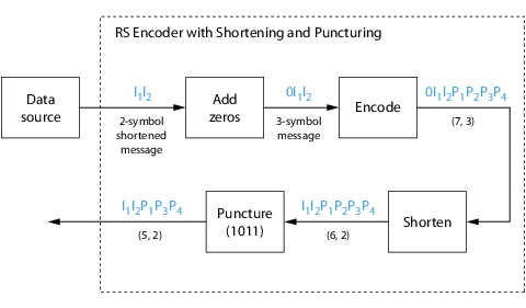
The following figure shows a representative example of a (7,3) Reed Solomon encoder with shortening and puncturing.
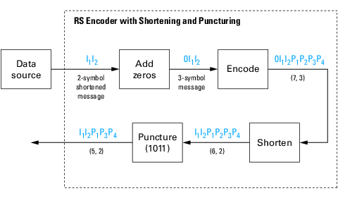
In this figure, the message source outputs two information symbols, designated by I1I2. (For a BCH example, the symbols are binary bits.) Because the code is a shortened (7,3) code, a zero must be added ahead of the information symbols, yielding a three-symbol message of 0I1I2. The modified message sequence is RS encoded, and the added information zero is then removed, which yields a result of I1I2P1P2P3P4. (In this example, the parity bits are at the end of the codeword.)
The puncturing operation is governed by the puncture vector, which, in this case,
is 1011. Within the puncture vector, a 1 means that the
symbol is kept, and a 0 means that the symbol is thrown away. In
this example, the puncturing operation removes the second parity symbol, yielding a
final vector of I1I2P1P3P4.
Decoder Example with Shortening and Puncturing
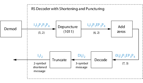
The following figure shows how the RS decoder operates on a shortened and punctured codeword.
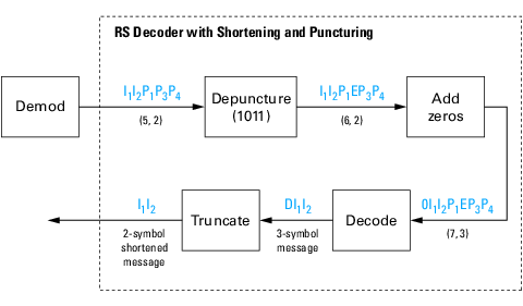
This case corresponds to the encoder operations shown in the figure of the RS encoder with shortening and puncturing. As shown in the preceding figure, the encoder receives a (5,2) codeword, because it has been shortened from a (7,3) codeword by one symbol, and one symbol has also been punctured.
As a first step, the decoder adds an erasure, designated by E, in the second parity position of the codeword. This corresponds to the puncture vector 1011. Adding a zero accounts for shortening, in the same way as shown in the preceding figure. The single erasure does not exceed the erasure-correcting capability of the code, which can correct four erasures. The decoding operation results in the three-symbol message DI1I2. The first symbol is truncated, as in the preceding figure, yielding a final output of I1I2.
Decoder Example with Shortening, Puncturing, and Erasures
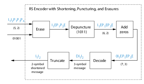
The following figure shows the decoder operating on the punctured, shortened codeword, while also correcting erasures generated by the receiver.

In this figure, demodulator receives the I1I2P1P3P4 vector that the encoder sent. The demodulator declares that two of the five received symbols are unreliable enough to be erased, such that symbols 2 and 5 are deemed to be erasures. The 01001 vector, provided by an external source, indicates these erasures. Within the erasures vector, a 1 means that the symbol is to be replaced with an erasure symbol, and a 0 means that the symbol is passed unaltered.
The decoder blocks receive the codeword and the erasure vector, and perform the erasures indicated by the vector 01001. Within the erasures vector, a 1 means that the symbol is to be replaced with an erasure symbol, and a 0 means that the symbol is passed unaltered. The resulting codeword vector is I1EP1P3E, where E is an erasure symbol.
The codeword is then depunctured, according to the puncture vector used in the encoding operation (i.e., 1011). Thus, an erasure symbol is inserted between P1 and P3, yielding a codeword vector of I1EP1EP3E.
Just prior to decoding, the addition of zeros at the beginning of the information vector accounts for the shortening. The resulting vector is 0I1EP1EP3E, such that a (7,3) codeword is sent to the Berlekamp algorithm.
This codeword is decoded, yielding a three-symbol message of DI1I2 (where D refers to a dummy symbol). Finally, the removal of the D symbol from the message vector accounts for the shortening and yields the original I1I2 vector.
For additional information, see the Reed-Solomon Coding with Erasures, Punctures, and Shortening MATLAB example or the Reed-Solomon Coding with Erasures, Punctures, and Shortening in Simulink example.
Reed-Solomon Code in Integer Format
For a model that uses a Reed-Solomon code in integer format, see the Integer-Output RS Decoder block reference page.
Find Generator Polynomial for Cyclic, BCH, or RS Codes
To find a generator polynomial for a cyclic, BCH, or Reed-Solomon code, use the cyclpoly, bchgenpoly, or rsgenpoly function, respectively.
Find Generator Polynomials
Use these commands to find generator polynomials for block codes of different types.
genpolyCyclic = cyclpoly(15,5) % 1+X^5+X^10genpolyCyclic = 1×11
1 0 0 0 0 1 0 0 0 0 1
genpolyBCH = bchgenpoly(15,5) % x^10+x^8+x^5+x^4+x^2+x+1genpolyBCH = GF(2) array. Array elements = 1 0 1 0 0 1 1 0 1 1 1
genpolyRS = rsgenpoly(15,5)
genpolyRS = GF(2^4) array. Primitive polynomial = D^4+D+1 (19 decimal)
Array elements =
1 4 8 10 12 9 4 2 12 2 7
The formats of these outputs vary:
cyclpolyrepresents a generator polynomial using an integer row vector that lists the polynomial's coefficients in order of ascending powers of the variable.bchgenpolyandrsgenpolyrepresent a generator polynomial using a Galois row vector that lists the polynomial's coefficients in order of descending powers of the variable.rsgenpolyuses coefficients in a Galois field other than the binary field GF(2). For more information on the meaning of these coefficients, see How Integers Correspond to Galois Field Elements and Polynomials over Galois Fields.
Nonuniqueness of Generator Polynomials
Some pairs of message length and codeword length do not uniquely determine the generator polynomial. Syntaxes for functions above also include options for retrieving generator polynomials that satisfy certain constraints that you specify. See the cyclpoly, bchgenpoly, or rsgenpoly function reference pages for details about syntax options.
Algebraic Expression for Generator Polynomials
The generator polynomials produced by bchgenpoly and rsgenpoly have the form: , where A is a primitive element for an appropriate Galois field, and b and t are integers. See the bchgenpoly and rsgenpoly function reference pages for more information about this expression.
Performing Other Block Code Tasks
This section describes functions that compute typical parameters associated with linear block codes, as well as functions that convert information from one format to another.
Error Correction Versus Error Detection for Linear Block Codes
You can use a linear block code to detect dmin – 1 errors or to correct errors.
If you compromise the error correction capability of a code, you can detect more than t errors. For example, a code with dmin = 7 can correct t = 3 errors or it can detect up to 4 errors and correct up to 2 errors.
Find BCH and RS Code Error-Correction Capability
The bchgenpoly and rsgenpoly functions can return an optional second output argument that indicates the error-correction capability of a BCH or Reed-Solomon code.
This command shows that a [31,16] BCH code can correct up to three errors in each codeword.
[g1,t1] = bchgenpoly(31,16); t1
t1 = 3
This command shows that a [31,16] RS code can correct up to seven errors in each codeword.
[g2,t2] = rsgenpoly(31,16); t2
t2 = 7
Find Hamming and Cyclic Code Parity-Check and Generator Matrices
The hammgen and cyclgen functions return the parity-check and generator matrix for Hamming and cyclic codes, respectively.
Hamming Code Parity-Check and Generator Matrices
To find a parity-check and generator matrix for a Hamming code with codeword length , use the hammgen function. m must be at least 3. For example,
m=3;
[parmat,genmat] = hammgen(m) % Hammingparmat = 3×7
1 0 0 1 0 1 1
0 1 0 1 1 1 0
0 0 1 0 1 1 1
genmat = 4×7
1 1 0 1 0 0 0
0 1 1 0 1 0 0
1 1 1 0 0 1 0
1 0 1 0 0 0 1
Cyclic Code Parity-Check and Generator Matrices
To find a parity-check and generator matrix for a cyclic code, use the cyclgen function. You must provide the codeword length and a valid generator polynomial. You can use the cyclpoly function to produce one possible generator polynomial after you provide the codeword length and message length. For example,
[parmat,genmat] = cyclgen(7,cyclpoly(7,4)) % Cyclicparmat = 3×7
1 0 0 1 1 1 0
0 1 0 0 1 1 1
0 0 1 1 1 0 1
genmat = 4×7
1 0 1 1 0 0 0
1 1 1 0 1 0 0
1 1 0 0 0 1 0
0 1 1 0 0 0 1
Converting Between Parity-Check and Generator Matrices
The gen2par function converts a generator matrix into a parity-check matrix, and vice versa.
Selected Bibliography for Block Coding
[1] Berlekamp, Elwyn R., Algebraic Coding Theory, New York, McGraw-Hill, 1968.
[2] Clark, George C., and J. Bibb Cain. Error-Correction Coding for Digital Communications. Applications of Communications Theory. New York: Plenum Press, 1981.
[3] Lin, Shu, and Daniel J. Costello, Jr., Error Control Coding: Fundamentals and Applications, Englewood Cliffs, NJ, Prentice-Hall, 1983.
[4] Peterson, W. Wesley, and E. J. Weldon. Error-Correcting Codes. 2d ed. MIT Press, 1972.
[5] van Lint, J. H., Introduction to Coding Theory, New York, Springer-Verlag, 1982.
[6] Wicker, Stephen B. Error Control Systems for Digital Communication and Storage. Upper Saddle River, NJ: Prentice Hall, 1995.
[7] Gallager, Robert G. Low-Density Parity-Check Codes. Cambridge, MA: MIT Press, 1963.
[8] Ryan, William E., “An introduction to LDPC codes,” Coding and Signal Processing for Magnetic Recoding Systems (Vasic, B., ed.), CRC Press, 2004.
[9] Blahut, Richard E. Algebraic Codes for Data Transmission. Cambridge University Press, 2003.
Linear Block Codes
Represent Words for Linear Block Codes
Communication Toolbox® functionality for cyclic, Hamming, and generic linear block coding offers you multiple ways to organize bits in messages or codewords. This example uses the encode function to create messages and codewords in these formats:
Binary vector - messages and codewords can take the form of vectors containing 0s and 1s
Binary matrix - organizes coding information to emphasize the grouping of digits into messages and codewords
Decimal vector - messages and codewords can take the form of vectors containing integers
The examples use cyclic coding. Hamming and generic linear block codes use similar formats for messages and codes.
Create Messages and Codewords in Binary Vector Format
Your messages and codewords can take the form of vectors containing 0s and 1s. For example, generate [6,4] cyclic coded messages and codewords.
n = 6; % Codeword length k = 4; % Message length
Encode a column vector consisting of a 12-bit message, msg. The generated codeword, cw, is a binary column vector.
msg = [1 0 0 1 1 0 1 0 1 0 1 1]';
cw = encode(msg,n,k,'cyclic');Transpose and display the binary vectors msg and cw.
msg'
ans = 1×12
1 0 0 1 1 0 1 0 1 0 1 1
cw'
ans = 1×18
1 1 1 0 0 1 0 0 1 0 1 0 0 1 1 0 1 1
For k=4, the input message, msg, consists of 12 bits, which are interpreted as three 4-bit messages. Since n=6, the resulting vector codeword, cw, comprises three 6-bit codewords, which are concatenated to form a vector of length 18. The parity bits are at the beginning of each codeword.
Create Messages and Codewords in Binary Matrix Format
You can organize coding information to emphasize the grouping of digits into messages and codewords. With this approach, each message or codeword occupies a row in a binary matrix. The example below illustrates this approach by listing each 4-bit message on a distinct row in msg and each 6-bit codeword on a distinct row in cw.
Your messages and codewords can take the form of matrices containing 0s and 1s. For example, generate [6,4] cyclic coded messages and codewords.
n = 6; % Codeword length k = 4; % Message length
Initialize a binary message, msg, in a 3-by-4 matrix. Using a [6,4] cyclic code, the encoder generates a 3-by-6 matrix of binary codewords.
msg = [1 0 0 1; 1 0 1 0; 1 0 1 1];
cw = encode(msg,n,k,'cyclic');
msgmsg = 3×4
1 0 0 1
1 0 1 0
1 0 1 1
cw
cw = 3×6
1 1 1 0 0 1
0 0 1 0 1 0
0 1 1 0 1 1
In the binary matrix format, the message matrix must have k columns. The corresponding code matrix has n columns. The parity bits are at the beginning of each row.
Create Messages and Codewords in Decimal Vector Format
Your messages and codewords can take the form of vectors containing integers. Each element of the vector gives the decimal representation of the bits in one message or one codeword. When encoding in decimal vector format, keep in mind that:
Since the
encodefunction uses a binary format internally, when your coding involves very large or , using the default binary format instead of decimal format avoids significant roundoff errors associated with converting many bits to large decimal numbers and back.When you use the decimal vector format, the
encodefunction expects the leftmost bit to be the least significant bit.When you input a decimal message, you must append
/decimalto the fourth argument when executing theencodefunction.
Define the codeword and message lengths. Generate message, msg, as a decimal column vector. The syntax for the encode function must mention the decimal format explicitly.
n = 6; % Codeword length k = 4; % Message length msg = [9;5;13];
The function outputs cw as a decimal vector of codewords.
cw = encode(msg,n,k,'cyclic/decimal')cw = 3×1
39
20
54
Configure Parameters for Linear Block Codes
This subsection describes the items that you might need in order to process [n,k] cyclic, Hamming, and generic linear block codes. This table lists the items and the coding techniques for which they are most relevant.
Parameters Used in Block Coding Techniques
| Parameter | Block Coding Technique |
|---|---|
| Generator Matrix | Generic linear block |
| Parity-Check Matrix | Generic linear block |
| Generator Polynomial for Cyclic Coding | Cyclic |
| Use Decoding Table in MATLAB | Generic linear block, Hamming |
Generator Matrix. The process of encoding a message into an [n,k] linear block code is determined by a k-by-n generator matrix G. Specifically, the 1-by-k message vector v is encoded into the 1-by-n codeword vector vG. If G has the form [Ik P] or [P Ik], where P is some k-by-(n-k) matrix and Ik is the k-by-k identity matrix, G is said to be in standard form. Some authors, such as Clark and Cain [2], use the first standard form. Others authors, such as Lin and Costello [3], use the second. Most functions in Communications Toolbox assume that a generator matrix is in standard form when you use it as an input argument.
The Parity-Check Matrix section shows examples of generator matrices.
Parity-Check Matrix. Decoding an [n,k] linear block code requires an (n–k)-by-n parity-check matrix H. It satisfies GHtr = 0 (mod 2), where Htr denotes the matrix transpose of H, G is the generator matrix of the code, and this zero matrix is k-by-(n–k). If G = [IkP] then H = [–PtrIn–k]. Most functions in this product assume that a parity-check matrix is in standard form when you use it as an input argument.
This table summarizes the standard forms of generator and parity-check matrices for an [n–k] binary linear block code.
| Type of Matrix | Standard Form | Dimensions |
|---|---|---|
| Generator | [IkP] or [PIk] | k-by-n |
| Parity-check | [–P'In–k] or [In–k–P'] | (n–k)-by-n |
Ik is the identity matrix of size k and the ' symbol indicates matrix transpose.
Note
For binary codes, the minus signs in the parity-check form listed above are irrelevant; that is, –1 = 1 in the binary field.
Create Parity-Check and Generator Matrices
In the commands below, parmat is a parity-check matrix and genmat is a generator matrix.
This code finds parity-check and generator matrices for an Hamming code, in which , by using the hammgen function. genmat has the standard form .
[parmat,genmat] = hammgen(3)
parmat = 3×7
1 0 0 1 0 1 1
0 1 0 1 1 1 0
0 0 1 0 1 1 1
genmat = 4×7
1 1 0 1 0 0 0
0 1 1 0 1 0 0
1 1 1 0 0 1 0
1 0 1 0 0 0 1
This code finds parity-check and generator matrices for a [7,3] cyclic code by using the cyclpoly and cyclgen functions.
genpoly = cyclpoly(7,3); [parmat,genmat] = cyclgen(7,genpoly)
parmat = 4×7
1 0 0 0 1 1 0
0 1 0 0 0 1 1
0 0 1 0 1 1 1
0 0 0 1 1 0 1
genmat = 3×7
1 0 1 1 1 0 0
1 1 1 0 0 1 0
0 1 1 1 0 0 1
This code converts a generator matrix for a [5,3] linear block code into the corresponding parity-check matrix by using the gen2par function. The gen2par function can also convert a parity-check matrix into a generator matrix.
genmat = [1 0 0 1 0; 0 1 0 1 1; 0 0 1 0 1]; parmat = gen2par(genmat)
parmat = 2×5
1 1 0 1 0
0 1 1 0 1
Generator Polynomial for Cyclic Coding
Cyclic codes have algebraic properties that allow a polynomial to determine the coding process completely. This so-called generator polynomial is a degree-(n–k) divisor of the polynomial . Van Lint [5] explains how a generator polynomial determines a cyclic code.
The cyclpoly function produces generator polynomials for cyclic codes that represent the generator polynomial using a row vector containing the polynomial coefficients in order of ascending powers of the variable. For example, this command finds that one valid generator polynomial for a [7,3] cyclic code is .
genpoly = cyclpoly(7,3)
genpoly = 1×5
1 0 1 1 1
Use Decoding Table in MATLAB
A decoding table tells a decoder how to correct errors that have corrupted the code during transmission. Hamming codes can correct any single-symbol error in any codeword. Other codes can correct or partially correct errors that corrupt more than one symbol in a codeword.
The Communications toolbox represents a decoding table as a matrix with n columns and rows. Each row gives a correction vector for one received codeword vector. A Hamming decoding table has n+1 rows. The syndtable function generates a decoding table for a given parity-check matrix.
This example uses a Hamming decoding table to correct an error in a received message. The hammgen function produces the parity-check matrix and the syndtable function produces the decoding table. To determine the syndrome, multiply the transpose of the parity-check matrix by the received codeword. The decoding table helps determine the correction vector. The corrected codeword is the sum (modulo 2) of the correction vector and the received codeword.
Set parameters for a [7,4] Hamming code.
m = 3; n = 2^m-1; k = n-m;
Produce a parity-check matrix and decoding table.
parmat = hammgen(m); trt = syndtable(parmat);
Specify a vector of received data.
recd = [1 0 0 1 1 1 1]
recd = 1×7
1 0 0 1 1 1 1
Calculate the syndrome and then display the decimal and binary values for the syndrome.
syndrome = rem(recd * parmat',2); syndrome_int = bit2int(syndrome',m); % Convert to decimal. disp(['Syndrome = ',num2str(syndrome_int), ... ' (decimal), ',num2str(syndrome),' (binary)'])
Syndrome = 3 (decimal), 0 1 1 (binary)
Determine the correction vector by using the decoding table and syndrome, and then compute the corrected codeword by using the correction vector.
corrvect = trt(1+syndrome_int,:)
corrvect = 1×7
0 0 0 0 1 0 0
correctedcode = rem(corrvect+recd,2)
correctedcode = 1×7
1 0 0 1 0 1 1
Create and Decode Linear Block Codes
The functions for encoding and decoding cyclic, Hamming, and generic linear
block codes are encode and decode.
This section discusses how to use these functions to create and decode generic linear block
codes, cyclic codes, and
Hamming
codes.
Generic Linear Block Codes. Encoding a message using a generic linear block code requires a generator
matrix. If you have defined variables msg,
n, k, and
genmat, either of the commands
code = encode(msg,n,k,'linear',genmat); code = encode(msg,n,k,'linear/decimal',genmat);
encodes the information in msg using the
[n,k] code that the generator
matrix genmat determines. The /decimal
option, suitable when 2^n and 2^k are
not very large, indicates that msg contains nonnegative
decimal integers rather than their binary representations. See Represent Words for Linear Block Codes or the reference page
for encode for a description of
the formats of msg and code.
Decoding the code requires the generator matrix and possibly a decoding
table. If you have defined variables code,
n, k, genmat,
and possibly also trt, then the commands
newmsg = decode(code,n,k,'linear',genmat); newmsg = decode(code,n,k,'linear/decimal',genmat); newmsg = decode(code,n,k,'linear',genmat,trt); newmsg = decode(code,n,k,'linear/decimal',genmat,trt);
decode the information in code, using the
[n,k] code that the generator
matrix genmat determines. decode
also corrects errors according to instructions in the decoding table that
trt represents.
Example: Generic Linear Block Coding
The example below encodes a message, artificially adds some noise, decodes the noisy code, and keeps track of errors that the decoder detects along the way. Because the decoding table contains only zeros, the decoder does not correct any errors.
n = 4; k = 2; genmat = [[1 1; 1 0], eye(2)]; % Generator matrix msg = [0 1; 0 0; 1 0]; % Three messages, two bits each % Create three codewords, four bits each. code = encode(msg,n,k,'linear',genmat); noisycode = rem(code + randerr(3,4,[0 1;.7 .3]),2); % Add noise. trt = zeros(2^(n-k),n); % No correction of errors % Decode, keeping track of all detected errors. [newmsg,err] = decode(noisycode,n,k,'linear',genmat,trt); err_words = find(err~=0) % Find out which words had errors.
The output indicates that errors occurred in the first and second words. Your results might vary because this example uses random numbers as errors.
err_words =
1
2
Cyclic Codes. A cyclic code is a linear block code with the property that cyclic shifts of a codeword (expressed as a series of bits) are also codewords. An alternative characterization of cyclic codes is based on its generator polynomial, as mentioned in Generator Polynomial for Cyclic Coding and discussed in [5].
Encoding a message using a cyclic code requires a generator polynomial. If
you have defined variables msg, n,
k, and genpoly, then either of the
commands
code = encode(msg,n,k,'cyclic',genpoly); code = encode(msg,n,k,'cyclic/decimal',genpoly);
encodes the information in msg using the
[n,k] code determined by the
generator polynomial genpoly. genpoly
is an optional argument for encode. The default
generator polynomial is cyclpoly(n,k). The
/decimal option, suitable when 2^n
and 2^k are not very large, indicates that
msg contains nonnegative decimal integers rather than
their binary representations. See Represent Words for Linear Block Codes or the reference page
for encode for a description of
the formats of msg and code.
Decoding the code requires the generator polynomial and possibly a
decoding table. If you have defined variables code,
n, k, genpoly,
and trt, then the commands
newmsg = decode(code,n,k,'cyclic',genpoly); newmsg = decode(code,n,k,'cyclic/decimal',genpoly); newmsg = decode(code,n,k,'cyclic',genpoly,trt); newmsg = decode(code,n,k,'cyclic/decimal',genpoly,trt);
decode the information in code, using the
[n,k] code that the generator
matrix genmat determines. decode
also corrects errors according to instructions in the decoding table that
trt represents. genpoly is an
optional argument in the first two syntaxes above. The default generator
polynomial is cyclpoly(n,k).
Example
You can modify the example in Generic Linear Block Codes
so that it uses the cyclic coding technique, instead of the linear block
code with the generator matrix genmat. Make the changes
listed below:
Replace the second line by
genpoly = [1 0 1]; % generator poly is 1 + x^2In the fifth and ninth lines (
encodeanddecodecommands), replacegenmatbygenpolyand replace'linear'by'cyclic'.
Another example of encoding and decoding a cyclic code is on the reference
page for encode.
Hamming Codes. The reference pages for encode and decode contain examples of
encoding and decoding Hamming codes. Also, the Use Decoding Table in MATLAB section illustrates error
correction in a Hamming code.
BCH Codes
Represent Words for BCH Codes
A message for an [N,K] BCH code must be a K-column binary Galois field array. The code that corresponds to that message is an N-column binary Galois field array. Each row of these Galois field arrays represents one word.
This example illustrates the representation of message and code words for a [15, 11] BCH code.
msg = [1 0 0 1 0; 1 0 1 1 1]; % Messages in a Galois array
bchenc = comm.BCHEncoder;
c1 = bchenc(msg(1,:)');
c2 = bchenc(msg(2,:)');Concatenate and transpose the results to conveniently display the encoded output.
c = [c1 c2]'
c = 2×15
1 0 0 1 0 0 0 1 1 1 1 0 1 0 1
1 0 1 1 1 0 0 0 0 1 0 1 0 0 1
Parameters for BCH Codes
BCH codes use special values of n and
k:
n, the codeword length, is an integer of the form 2m-1 for some integer m > 2.k, the message length, is a positive integer less thann. However, only some positive integers less thannare valid choices fork. See the BCH Encoder block reference page for a list of some valid values ofkcorresponding to values ofnup to 511.
Create and Decode BCH Codes
The BCH Encoder and BCH Decoder System objects create and decode BCH codes, using the
data described in Represent Words for BCH Codes and Parameters for BCH Codes.
Parity Symbol Positioning for BCH Codes
The convention used in Communications Toolbox appends parity symbols to BCH codes. This example encodes and decodes a [15,5] BCH code with parity symbols appended. It also shows you how to convert encoded data with appended parity symbols to encoded data with prepended parity symbols.
Define the codeword and message lengths, and then generate four random binary message frames in a column vector.
n = 15; % Codeword length k = 5; % Message length Nmsg = 4; % Number of frames msg = randi([0 1],4*k,1); % Random binary messages
BCH Coding
Encode and decode by using default [15,5] BCH encode and decode System objects. BCH encoding appends parity symbols to each codeword and concatenates the coded result to output a column vector. The BCH decoding removes the coding and parity symbols.
bchenc = comm.BCHEncoder(n,k); bchdec = comm.BCHDecoder(n,k); c1 = bchenc(msg); d1 = bchdec(c1);
Check that the decoding worked correctly.
chk = isequal(d1,msg)
chk = logical
1
BCH Coding with Prepended Parity Symbols
To perform the BCH encoding and decoding operations with prepended parity symbols, use the reshape and circshift functions to manipulate the data after encoding. Use the reshape function to separate the input vector into a matrix storing each codeword in a column. Use the circshift function to move the appended parity symbols from the end of each codeword to prepended parity symbols at the beginning of each codeword. Convert the matrix back to a column vector for transmission.
c11 = reshape(c1,n,[]); c12 = circshift(c11,n-k); c1_prepend = c12(:);
Decode BCH with Prepended Parity Symbols
To decode the BCH code with prepended parity symbols, convert the received data with prepended parity symbols to data with appended parity symbols. Use the reshape and circshift functions to manipulate the data again. Use the reshape function to separate the input vector into a matrix storing each codeword in a column. Use the circshift function to move the prepended parity symbols from the beginning of the codeword to appended parity symbols at the end of the codeword.
c21 = reshape(c1_prepend,n,[]); c22 = circshift(c21,k); c1_append = c22(:);
Decode and check that the prepend-to-append conversion worked correctly.
d1_append = bchdec(c1_append); chk = isequal(msg,d1_append)
chk = logical
1
Detect and Correct Errors in BCH Code Using MATLAB
This example shows the decoding results for a corrupted [15,5] BCH code. The example encodes data, introduces errors in each codeword, and attempts to decode the noisy code.
Define parameters for a [15,5] BCH code and four random K-symbol message words. Create a [15,5] BCH generator polynomial and output the error correction capability of a [15,5] BCH code as t.
N = 15; % Codeword length K = 5; % Message length nw = 4; % Number of words to process msgw = randi([0 1], nw*K, 1); % Random k-symbol messages [gp,t] = bchgenpoly(N,K); % t is error-correction capability t
t = 3
Create [15,5] BCH encoder and decoder System objects.
bchenc = comm.BCHEncoder(N,K, ... GeneratorPolynomialSource='Property', ... GeneratorPolynomial=gp); bchdec = comm.BCHDecoder(N,K, ... GeneratorPolynomialSource='Property', ... GeneratorPolynomial=gp);
Encode the message data.
cw = bchenc(msgw);
Generate random noise that inserts t errors per codeword. Notice that the array of noise values contains binary values, and that the adding noise to the code (cw + noise) takes place in the Galois field GF(2) because cw is a Galois field array in GF(2).
noise = randerr(nw,N,t); noisy = noise'; noisy = noisy(:);
Add the noise vector to the binary code by using the mod function. Decode the noisy data and output the number of errors corrected in each codeword. The values in the vector nerrs indicate that the decoder corrected t errors in each codeword. Check to confirm the decoding working correctly, by using the isequal function. The nonzero value returned indicates that the decoder was able to correct the corrupted codewords and recover the original message.
cwnoisy = mod(cw + noisy,2); [dcw, nerrs] = bchdec(cwnoisy); nerrs
nerrs = 4×1
3
3
3
3
chk2 = isequal(dcw,msgw)
chk2 = logical
1
Each BCH code has a finite error-correction capability. To learn more about how the comm.BCHDecoder System object™ behaves when the noise is excessive and causes more errors than the code is capable of correcting, see the analogous discussion for Reed-Solomon codes in Detect and Correct Errors in Reed-Solomon Code Using MATLAB.
Algorithms for BCH and RS Errors-only Decoding
Overview. The errors-only decoding algorithm used for BCH and RS codes can be described by the following steps (sections 5.3.2, 5.4, and 5.6 in [2]).
Calculate the first 2t terms of the infinite degree syndrome polynomial, .
If those 2t terms of are all equal to 0, then the code has no errors , no correction needs to be performed, and the decoding algorithm ends.
If one or more terms of are nonzero, calculate the error locator polynomial, Λ(z), via the Berlekamp algorithm.
Calculate the error evaluator polynomial, , via
Correct an error in the codeword according to
where is the error magnitude in the th position in the codeword, m is a value less than the error-correcting capability of the code, is the error magnitude polynomial, Λ'(z) is the formal derivative [6] of the error locator polynomial, Λ(z), and α is the primitive element of the Galois field of the code.
Further description of several of the steps is given in the following sections.
Syndrome Calculation. For narrow-sense codes, the 2t terms of are calculated by evaluating the received codeword at successive powers of α (the field’s primitive element) over the range [0, (2t–1)]. In other words, if you assume one-based indexing of codewords and the syndrome polynomial , and that codewords are of the form , then each term of is given as
Error Locator Polynomial Calculation. The error locator polynomial, Λ(z), is found using the Berlekamp algorithm. This diagram shows an iterative procedure to find Λ(z) by using the Berlekamp algorithm.
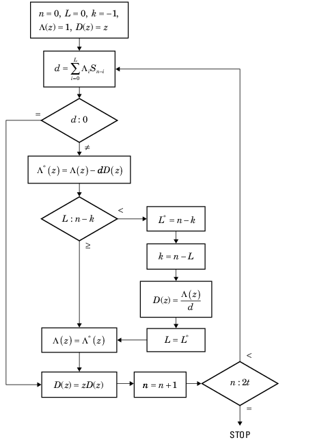
| Variable | Description |
|---|---|
| n | Iterator variable |
| k | Iterator variable |
| L | Length of the feedback register used to generate the first 2t terms of |
| D(z) | Correction polynomial |
| d | Discrepancy |
For a detailed description of the error locator polynomial calculation algorithm, see [2].
Error Evaluator Polynomial Calculation. The error evaluator polynomial, , is simply the convolution of Λ(z) and .
Hamming Codes
Create Hamming Code in Binary Format Using Simulink
This example shows how to model a simple encoder and decoder using appropriate vector lengths for the code and message.
The cm_hamming model includes these blocks:
Bernoulli Binary Generator block with
Samples per frameset to4to match the Hamming encoder message lengthHamming Encoder block with default parameter values
Hamming Decoder block with default parameter values
Error Rate Calculation block with
Output dataset toPortDisplay block connected to the output port of the Error Rate Calculation block
To display the vector length of signals in the model, go to Debug > Diagnostics > Information Overlays > Signals and select Signal Dimensions. The connector lines show the signal attributes. To compile the model, press Ctrl+D. Run the model to display the error rate statistics.
Reduce the Error Rate Using a Hamming Code
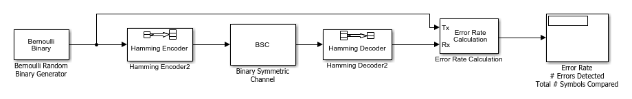
This section describes how to reduce the error rate by adding an error-correcting code. This figure shows a model that uses Hamming coding.
Building the Hamming Code Model
Build the Hamming code model and save the model as
my_hamming in the folder where you keep your work files
by following these steps:
Open a new model window and expand the window area as desired to accommodate the model. Type block names in the model window and add Bernoulli Binary Generator, Hamming Encoder, Binary Symmetric Channel, Hamming Decoder, Error Rate Calculation, and Display (Simulink) blocks:
Arrange and connect the blocks to create a model that resemble this one.
Using the Hamming Encoder and Decoder Blocks
The Hamming Encoder block encodes the data before it is sent through the channel. The default code is the [7,4] Hamming code, which encodes message words of length 4 into codewords of length 7. As a result, the block converts frames of size 4 into frames of size 7. The code can correct one error in each transmitted codeword.
For an [n,k] code, the input to the Hamming Encoder block must consist of vectors of size k. In this example, k = 4.
The Hamming Decoder block decodes the data after it is sent through the channel. If at most one error is created in a codeword by the channel, the block decodes the word correctly. However, if more than one error occurs, the Hamming Decoder block might decode incorrectly.
To learn more about block coding features, see Block Codes.
Setting Parameters in the Hamming Code Model
Double-click the Bernoulli Binary Generator block and make the following changes to the parameter settings in the block's dialog box, as shown in the following figure:
Set Samples per frame to
4. This converts the output of the block into frames of size 4, in order to meet the input requirement of the Hamming Encoder Block. See Sample-Based and Frame-Based Processing for more information about frames.Note
Many blocks, such as the Hamming Encoder block, require their input to be a vector of a specific size. If you connect a source block, such as the Bernoulli Binary Generator block, to one of these blocks, set Samples per frame to the required value. For this model the Samples per frame parameter of the Bernoulli Binary Generator block must be a multiple of the Message Length K parameter of the Hamming Encoder block.
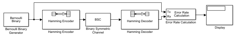
Labeling the Display Block
You can change the label that appears below a block to make it more
informative. For example, to change the label below the Display block to
'Error Rate Display', first select the label with the
mouse. This causes a box to appear around the text. Enter the changes to the
text in the box.
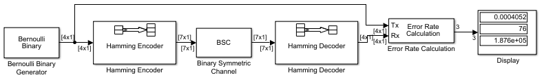
Running the Hamming Code Model
To run the model, select Simulation > Run. The model terminates after 100 errors occur. The error rate, displayed in the top window of the Display block, is approximately .001. You get slightly different results if you change the Initial seed parameters in the model or run a simulation for a different length of time.
You expect an error rate of approximately .001 for the following reason: The probability of two or more errors occurring in a codeword of length 7 is
| 1 – (0.99)7 – 7(0.99)6(0.01) = 0.002 | (1) |
If the codewords with two or more errors are decoded randomly, you expect about half the bits in the decoded message words to be incorrect. This indicates that .001 is a reasonable value for the bit error rate.
To obtain a lower error rate for the same probability of error, try using a Hamming code with larger parameters. To do this, change the parameters Codeword length and Message length in the Hamming Encoder and Hamming Decoder block dialog boxes. You also have to make the appropriate changes to the parameters of the Bernoulli Binary Generator block and the Binary Symmetric Channel block.
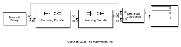
Displaying Frame Sizes
You can display the sizes of data frames in different parts in your model. On
the Debug tab, expand Information
Overlays. In the Signals section,
select Signal Dimensions. The line leading out of the
Bernoulli Binary Generator block is labeled
[4x1], indicating that its output consists of column
vectors of size 4. Because the Hamming Encoder block uses a [7,4]
code, it converts frames of size 4 into frames of size 7, so its output is
labeled [7x1].
Adding a Scope to the Model
To display the channel errors produced by the Binary Symmetric Channel block, add a Scope block to the model. This is a good way to see whether your model is functioning correctly. The example shown in the following figure shows where to insert the Scope block into the model.
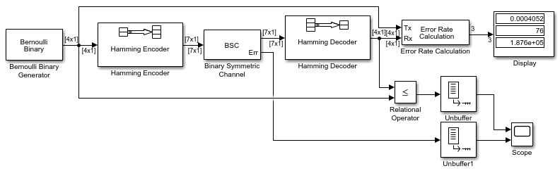
To build this model from the one shown in the figure Reduce the Error Rate Using a Hamming Code, follow these steps:
Type block names in the model window and add these blocks:
Relational Operator (Simulink)
Scope (Simulink)
Two copies of the Unbuffer
Double-click the Binary Symmetric Channel block to open its dialog box, and select Output error vector. This creates a second output port for the block, which carries the error vector.
Double-click the Scope block, under View > Configuration Properties, set Number of input ports to
2. Select Layout and highlight two blocks vertically. Click OK.Connect the blocks as shown in the preceding figure.
Setting Parameters in the Expanded Model
Make the following changes to the parameters for the blocks you added to the model.
Error Rate Calculation Block – Double-click the Error Rate Calculation block and clear the box next to Stop simulation in the block's dialog box.
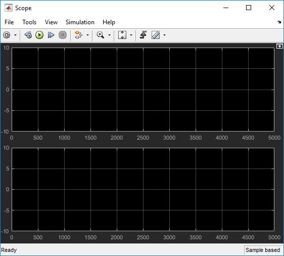
Scope Block – The Scope (Simulink) block displays the channel errors and uncorrected errors. To configure the block,
Double-click the Scope block, select View > Configuration Properties.
Select the Time tab and set Time span to
5000.Select the Logging tab and set Limit data points to last to
30000.Click OK.
The scope should now appear as shown.
To configure the axes, follow these steps:
Right-click the vertical axis at the left side of the upper scope.
In the context menu, select Configuration Properties.
Set Y-limits (Minimum) to
-1.Set Y-limits (Maximum) to
2, and click OK.Repeat the same steps for the vertical axis of the lower scope.
Widen the scope window until it is roughly three times as wide as it is high. You can do this by clicking the right border of the window and dragging the border to the right, while pressing the left-mouse button.
Relational Operator – Set Relational Operator to
~=in the block's dialog box. The Relational Operator block compares the transmitted signal, coming from the Bernoulli Random Generator block, with the received signal, coming from the Hamming Decoder block. The block outputs a 0 when the two signals agree and a 1 when they disagree.
Observing Channel Errors with the Scope
When you run the model, the scope displays the error data. At the end of each 5000 time steps, the scope appears as shown this figure. The scope then clears the displayed data and displays the next 5000 data points.
The upper scope shows the channel errors generated by the Binary Symmetric Channel block. The lower scope shows errors that are not corrected by channel coding.
Click the Stop button on the toolbar at the top of the model window to stop the scope.
You can see individual errors by zooming in on the scope. First click the middle magnifying glass button at the top left of the Scope window. Then click one of the lines in the lower scope. This zooms in horizontally on the line. Continue clicking the lines in the lower scope until the horizontal scale is fine enough to detect individual errors. A typical example of what you might see is shown in the figure below.
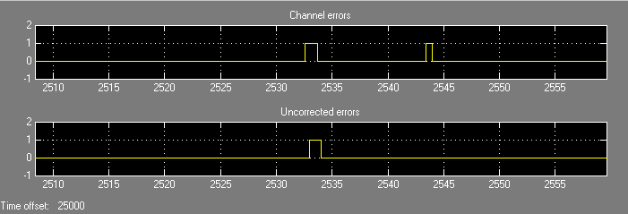
The wider rectangular pulse in the middle of the upper scope represents two 1s. These two errors, which occur in a single codeword, are not corrected. This accounts for the uncorrected errors in the lower scope. The narrower rectangular pulse to the right of the upper scope represents a single error, which is corrected.
When you are done observing the errors, select Simulation > Stop.
Export Data to MATLAB explains how to send the error data to the MATLAB workspace for more detailed analysis.
Reed-Solomon Codes
Represent Words for Reed-Solomon Codes
This toolbox supports Reed-Solomon codes that use m-bit symbols instead of
bits. A message for an [n,k] Reed-Solomon
code must be a k-column Galois field array in the field
GF(2m). Each array entry must be an integer
between 0 and 2m-1. The code corresponding to that
message is an n-column Galois field array in
GF(2m). The codeword length n
must be between 3 and 2m-1.
Note
For information about Galois field arrays and how to create them, see
Representing Elements of Galois Fields or the reference page
for the gf function.
The example below illustrates how to represent words for a [7,3] Reed-Solomon code.
n = 7; k = 3; % Codeword length and message length m = 3; % Number of bits in each symbol msg = [1 6 4; 0 4 3]; % Message is a Galois array. obj = comm.RSEncoder(n, k); c1 = step(obj, msg(1,:)'); c2 = step(obj, msg(2,:)'); c = [c1 c2].'
The output is
C =
1 6 4 4 3 6 3
0 4 3 3 7 4 7
Parameters for Reed-Solomon Codes
This section describes several integers related to Reed-Solomon codes and discusses how to find generator polynomials.
Allowable Values of Integer Parameters. The table below summarizes the meanings and allowable values of some
positive integer quantities related to Reed-Solomon codes as supported in
this toolbox. The quantities n and k
are input parameters for Reed-Solomon functions in this toolbox.
| Symbol | Meaning | Value or Range |
|---|---|---|
| m | Number of bits per symbol | Integer in the range [3 16] |
n | Number of symbols per codeword | Integer in the range [3 (2m–1)] |
k | Number of symbols per message | Positive integer less than
n, such that
n-k is even |
| t | Error-correction capability of the code | (n-k)/2 |
Generator Polynomial. The rsgenpoly function produces generator polynomials
for Reed-Solomon codes. rsgenpoly represents a
generator polynomial using a Galois row vector that lists the polynomial's
coefficients in order of descending powers of the
variable. If each symbol has m bits, the Galois row vector is in the field
GF(2m). For example, the command
r = rsgenpoly(15,13)
r = GF(2^4) array. Primitive polynomial = D^4+D+1 (19 decimal)
Array elements =
1 6 8
finds that one generator polynomial for a [15,13] Reed-Solomon code is X2 + (A2 + A)X + (A3), where A is a root of the default primitive polynomial for GF(16).
Algebraic Expression for Generator Polynomials
The generator polynomials that rsgenpoly produces
have the form
(X - Ab)(X - Ab+1)...(X - Ab+2t-1),
where b is an integer, A is a root of the primitive polynomial for the
Galois field, and t is (n-k)/2. The default value of b is
1. The output from rsgenpoly is the result of
multiplying the factors and collecting like powers of X. The example below
checks this formula for the case of a [15,13] Reed-Solomon code, using
b = 1.
n = 15; a = gf(2,log2(n+1)); % Root of primitive polynomial f1 = [1 a]; f2 = [1 a^2]; % Factors that form generator polynomial f = conv(f1,f2) % Generator polynomial, same as r above.
Create and Decode Reed-Solomon Codes
The comm.RSEncoder and comm.RSDecoder System objects
create and decode Reed-Solomon codes, using the data described in Represent Words for Reed-Solomon Codes and Parameters for Reed-Solomon Codes. This section illustrates how to
use the System objects.
Reed-Solomon Coding Syntaxes in MATLAB
This example shows multiple ways to encode and decode data using a [15,13] Reed-Solomon code. The example shows that you can:
Vary the generator polynomial for the code, using
rsgenpolyto produce a different generator polynomial.Vary the primitive polynomial for the Galois field that contains the symbols, using an input argument in
gf.Vary the position of the parity symbols within the codewords, choosing either the end (default) or beginning.
This example also shows that corresponding syntaxes of the comm.RSEncoder and comm.RSDecoder System objects use the same input arguments, except for the first input argument.
m = 4; % Number of bits in each symbol n = 2^m-1; % Codeword length k = 13; % Message length msg = randi([0 m-1],4*k,1); % Four random integer messages
The simplest syntax for encoding and decoding uses the default settings System object™ properties.
rsEnc = comm.RSEncoder(n,k); rsDec = comm.RSDecoder(n,k); c1 = rsEnc(msg); d1 = rsDec(c1);
Modify Generator Polynomial
Release the objects and modify the generator polynomial for the code.
release(rsEnc) release(rsDec) rsEnc.GeneratorPolynomialSource = 'Property'; rsDec.GeneratorPolynomialSource = 'Property'; rsEnc.GeneratorPolynomial = rsgenpoly(n,k,19,2); rsDec.GeneratorPolynomial = rsgenpoly(n,k,19,2); c2 = rsEnc(msg); d2 = rsDec(c2);
Modify Primitive Polynomial
Release the objects and modify the primitive polynomial for GF(16).
release(rsEnc) release(rsDec) rsEnc.PrimitivePolynomialSource = 'Property'; rsDec.PrimitivePolynomialSource = 'Property'; rsEnc.GeneratorPolynomialSource = 'Auto'; rsDec.GeneratorPolynomialSource = 'Auto'; rsEnc.PrimitivePolynomial = [1 1 0 0 1]; rsDec.PrimitivePolynomial = [1 1 0 0 1]; c3 = rsEnc(msg); d3 = rsDec(c3);
Check that the decoding worked correctly.
chk = isequal(d1,msg) & isequal(d2,msg) & isequal(d3,msg)
chk = logical
1
Appended Versus Prepended Parity Symbols
This code shows how to perform the encoding and decoding operations on a signal that has prepended parity symbols.
Convert encoded data with appended parity symbols to encoded data with prepended parity symbols by using the reshape and circshift functions.
c31 = reshape(c3,n,[]);
c32 = circshift(c31,n-k);
c3_prepend = c32(:); % RS encoded data with prepended parity symbols
The comm.RSDecoder System object expects parity symbols to be appended to the encoded signal. To decode the signal, you must convert the encoded data with prepended parity symbols to encoded data with appended parity symbols prior to decoding.
c34 = reshape(c3_prepend,n,[]);
c35 = circshift(c34,k);
c3_append = c35(:); % RS encoded data with appended parity symbols
Check that the prepend-to-append conversion worked correctly.
d3_append = rsDec(c3_append); chk = isequal(msg,d3_append)
chk = logical
1
Detect and Correct Errors in Reed-Solomon Code Using MATLAB
This example shows the decoding results for a corrupted code. The example encodes some data, introduces errors in each codeword, and then attempts to decode the noisy code by using the comm.RSDecoder System object™.
Correctable Noise Level in Reed-Solomon Codewords
Define parameters for the simulation and create RS encoder and decoder System objects. Compute the error correction capability, t, of the code.
m = 3; % Number of bits per symbol n = 2^m-1; % Codeword length k = 3; % Message length t = (n-k)/2 % Error-correction capability of the code
t = 2
nw = 4; % Number of words to process
rsEnc = comm.RSEncoder(n,k);
rsDec = comm.RSDecoder(n,k);Generate random k-symbol messages and encode the message.
msgw = randi([0 n],nw*k,1);
c = rsEnc(msgw); % Encode the data.Save the random number generator settings, and then to ensure repeatable results, specify a seed for the random number generator. Generate noise that adds t random errors per codeword. Add the noise to the code under gf(m) arithmetic, and then decode the noisy code. The array of noise values contains integers in the range , and the addition operation (c + noise) takes place in the Galois field because c is a Galois field array in .
s = rng; rng(123); noise = (1+randi([0 n-1],nw,n)).*randerr(nw,n,t); noisy = noise'; noisy = noisy(:); cnoisy = gf(c,m) + noisy; [dc nerrs] = rsDec(cnoisy.x);
Compare the decoded message, dc, to the original message, msgw, by using the isequal function. A return value of 1 indicates that dc and msgw match. The values in the vector nerrs indicate that the decoder corrected t errors in each codeword.
isequal(dc,msgw) % Confirm decoding worked correctlyans = logical
1
nerrs % Check number of errors corrected per codewordnerrs = 4×1 int32 column vector
2
2
2
2
Excessive Noise Level in Reed-Solomon Codewords
Each Reed-Solomon code has a finite error-correction capability. If the noise is so great that the corrupted codeword is too far in Hamming distance from the correct codeword, that means either:
The corrupted codeword is close to a valid codeword other than the correct codeword. The decoder returns the message that corresponds to the other codeword and is the incorrect decoding.
The corrupted codeword is not close enough to any codeword for successful decoding. This situation is called a decoding failure. The decoder removes the symbols in parity positions from the corrupted codeword and returns the remaining symbols.
In both cases, the decoder returns the wrong message. However, you can tell when a decoding failure occurs because RS decoder System object™ returns a value of –1 in its second output.
To examine cases in which codewords are too noisy for successful decoding, redefine the noise increasing t by one so that the number of errors per codeword exceeds the error correcting capability of the RS code. Decode (c + noise2) and check the results to show the decoding failure. Restore the random number generator settings.
noise2 = (1+randi([0 n-1],nw,n)).*randerr(nw,n,t+1); % t+1 errors/row noisy2 = noise2'; noisy2 = noisy2(:); cnoisy2 = gf(c,m) + noisy2; [dc2 nerrs2] = rsDec(cnoisy2.x); isequal(dc2,msgw) % Check whether decoding worked correctly
ans = logical
0
nerrs2 % Check number of errors corrected per codewordnerrs2 = 4×1 int32 column vector
-1
-1
-1
-1
rng(s)
Create Shortened Reed-Solomon Codes. Every Reed-Solomon encoder uses a codeword length that equals
2m-1 for an integer m. A shortened
Reed-Solomon code is one in which the codeword length is not
2m-1. A shortened
[n,k] Reed-Solomon code implicitly
uses an [n1,k1] encoder, where
n1 = 2m - 1, where m is the number of bits per symbol
k1 = k + (n1 - n)
The RS Encoder
System object supports shortened codes using the same syntaxes it uses for
nonshortened codes. You do not need to indicate explicitly that you want to
use a shortened code.
hEnc = comm.RSEncoder(7,5); ordinarycode = step(hEnc,[1 1 1 1 1]'); hEnc = comm.RSEncoder(5,3); shortenedcode = step(hEnc,[1 1 1 ]');
How the RS Encoder
System Object Creates a Shortened Code
When creating a shortened code, the RS
Encoder
System object performs these steps:
Pads each message by prepending zeros
Encodes each padded message using a Reed-Solomon encoder having an allowable codeword length and the desired error-correction capability
Removes the extra zeros from the nonparity symbols of each codeword
The following example illustrates this process.
n = 12; k = 8; % Lengths for the shortened code m = ceil(log2(n+1)); % Number of bits per symbol msg = randi([0 2^m-1],3*k,1); % Random array of 3 k-symbol words hEnc = comm.RSEncoder(n,k); code = step(hEnc, msg); % Create a shortened code. % Do the shortening manually, just to show how it works. n_pad = 2^m-1; % Codeword length in the actual encoder k_pad = k+(n_pad-n); % Messageword length in the actual encoder hEnc = comm.RSEncoder(n_pad,k_pad); mw = reshape(msg,k,[]); % Each column vector represents a messageword msg_pad = [zeros(n_pad-n,3); mw]; % Prepend zeros to each word. msg_pad = msg_pad(:); code_pad = step(hEnc,msg_pad); % Encode padded words. cw = reshape(code_pad,2^m-1,[]); % Each column vector represents a codeword code_eqv = cw(n_pad-n+1:n_pad,:); % Remove extra zeros. code_eqv = code_eqv(:); ck = isequal(code_eqv,code); % Returns true (1).
Find a Generator Polynomial
To find a generator polynomial for a cyclic, BCH, or Reed-Solomon code, use
the cyclpoly, bchgenpoly, or
rsgenpoly function, respectively. The commands
genpolyCyclic = cyclpoly(15,5) % 1+X^5+X^10 genpolyBCH = bchgenpoly(15,5) % x^10+x^8+x^5+x^4+x^2+x+1 genpolyRS = rsgenpoly(15,5)
find generator polynomials for block codes of different types. The output is below.
genpolyCyclic =
1 0 0 0 0 1 0 0 0 0 1
genpolyBCH = GF(2) array.

Array elements =

   1   0   1   0   0   1   1   0   1   1   1
genpolyRS = GF(2^4) array. Primitive polynomial = D^4+D+1 (19 decimal)

Array elements =

    1    4    8   10   12    9    4    2   12    2    7
The formats of these outputs vary:
cyclpolyrepresents a generator polynomial using an integer row vector that lists the polynomial's coefficients in order of ascending powers of the variable.bchgenpolyandrsgenpolyrepresent a generator polynomial using a Galois row vector that lists the polynomial's coefficients in order of descending powers of the variable.rsgenpolyuses coefficients in a Galois field other than the binary field GF(2). For more information on the meaning of these coefficients, see How Integers Correspond to Galois Field Elements and Polynomials over Galois Fields.
Nonuniqueness of Generator Polynomials. Some pairs of message length and codeword length do not uniquely determine the generator polynomial. The syntaxes for functions in the example above also include options for retrieving generator polynomials that satisfy certain constraints that you specify. See the functions' reference pages for details about syntax options.
Algebraic Expression for Generator Polynomials. The generator polynomials produced by bchgenpoly and
rsgenpoly have the form (X - Ab)(X - Ab+1)...(X - Ab+2t-1), where A is a primitive element for an
appropriate Galois field, and b and t
are integers. See the functions' reference pages for more information about
this expression.
Reed Solomon Examples with Shortening, Puncturing, and Erasures
In this section, a representative example of Reed Solomon coding with shortening, puncturing, and erasures is built with increasing complexity of error correction.
Encoder Example with Shortening and Puncturing. The following figure shows a representative example of a (7,3) Reed Solomon encoder with shortening and puncturing.
In this figure, the message source outputs two information symbols, designated by I1I2. (For a BCH example, the symbols are simply binary bits.) Because the code is a shortened (7,3) code, a zero must be added ahead of the information symbols, yielding a three-symbol message of 0I1I2. The modified message sequence is then RS encoded, and the added information zero is subsequently removed, which yields a result of I1I2P1P2P3P4. (In this example, the parity bits are at the end of the codeword.)
The puncturing operation is governed by the puncture vector, which, in this case, is 1011. Within the puncture vector, a 1 means that the symbol is kept, and a 0 means that the symbol is thrown away. In this example, the puncturing operation removes the second parity symbol, yielding a final vector of I1I2P1P3P4.
Decoder Example with Shortening and Puncturing. The following figure shows how the RS encoder operates on a shortened and punctured codeword.
This case corresponds to the encoder operations shown in the figure of the RS encoder with shortening and puncturing. As shown in the preceding figure, the encoder receives a (5,2) codeword, because it has been shortened from a (7,3) codeword by one symbol, and one symbol has also been punctured.
As a first step, the decoder adds an erasure, designated by E, in the second parity position of the codeword. This corresponds to the puncture vector 1011. Adding a zero accounts for shortening, in the same way as shown in the preceding figure. The single erasure does not exceed the erasure-correcting capability of the code, which can correct four erasures. The decoding operation results in the three-symbol message DI1I2. The first symbol is truncated, as in the preceding figure, yielding a final output of I1I2.
Encoder Example with Shortening, Puncturing, and Erasures. The following figure shows the decoder operating on the punctured, shortened codeword, while also correcting erasures generated by the receiver.
In this figure, demodulator receives the I1I2P1P3P4 vector that the encoder sent. The demodulator declares that two of the five received symbols are unreliable enough to be erased, such that symbols 2 and 5 are deemed to be erasures. The 01001 vector, provided by an external source, indicates these erasures. Within the erasures vector, a 1 means that the symbol is to be replaced with an erasure symbol, and a 0 means that the symbol is passed unaltered.
The decoder blocks receive the codeword and the erasure vector, and perform the erasures indicated by the vector 01001. Within the erasures vector, a 1 means that the symbol is to be replaced with an erasure symbol, and a 0 means that the symbol is passed unaltered. The resulting codeword vector is I1EP1P3E, where E is an erasure symbol.
The codeword is then depunctured, according to the puncture vector used in the encoding operation (i.e., 1011). Thus, an erasure symbol is inserted between P1 and P3, yielding a codeword vector of I1EP1EP3E.
Just prior to decoding, the addition of zeros at the beginning of the information vector accounts for the shortening. The resulting vector is 0I1EP1EP3E, such that a (7,3) codeword is sent to the Berlekamp algorithm.
This codeword is decoded, yielding a three-symbol message of DI1I2 (where D refers to a dummy symbol). Finally, the removal of the D symbol from the message vector accounts for the shortening and yields the original I1I2 vector.
For additional information, see the Reed-Solomon Coding with Erasures, Punctures, and Shortening in Simulink example.
LDPC Codes
Low-Density Parity-Check (LDPC) codes are linear error control codes with:
Sparse parity-check matrices
Long block lengths that can attain performance near the Shannon limit
Communications Toolbox supports LDPC coding using functions, objects, and blocks.
| Feature Type | Usage |
|---|---|
Functions: |
|
Configuration objects: | |
Blocks: LDPC Encoder and LDPC Decoder |
|
The LDPC decoding process is done iteratively. If the number of iterations is too small, the algorithm may not converge. You may need to experiment with the number of iterations to find an appropriate value for your model.
Unlike some other codecs, the LDPC decoder requires log-likelihood ratios (LLR). So, you cannot connect an LDPC decoder directly to the output of an LDPC encoder, but you can use a demodulator to compute the LLRs. Also, unlike other decoders, it is possible (although rare) that the output of the LDPC decoder does not satisfy all parity checks.
LDPC Decoding Algorithms
LDPC decoding uses one of these message-passing algorithms. The ldpcDecode function supports the belief propagation, layered
belief propagation, normalized min-sum, and offset min-sum decoding algorithms.
The LDPC Decoder block only supports the
belief propagation decoding algorithm.
Belief Propagation Decoding. The implementation of the belief propagation algorithm is based on the decoding algorithm presented by Gallager [2].
For transmitted LDPC-encoded codeword c = c0, c1, …, cn-1, the input to the LDPC decoder is the log-likelihood ratio (LLR) value .
In each iteration, the key components of the algorithm are updated based on these equations:
,
, initialized as before the first iteration, and
.
At the end of each iteration, L(Qi) contains the updated estimate of the LLR value for transmitted bit ci. The value L(Qi) is the soft-decision output for ci. If L(Qi) ≤ 0, the hard-decision output for ci is 1. Otherwise, the hard-decision output for ci is 0.
If decoding is configured to stop when all of the parity checks are satisfied, the algorithm verifies the parity-check equation (H c' = 0) at the end of each iteration. When all of the parity checks are satisfied, or if the maximum number of iterations is reached, decoding stops.
Index sets and are based on the parity-check matrix (PCM). Index sets Ci and Vj correspond to all nonzero elements in column i and row j of the PCM, respectively.
This figure shows the computation of these index sets in a given PCM for i = 5 and j = 3.
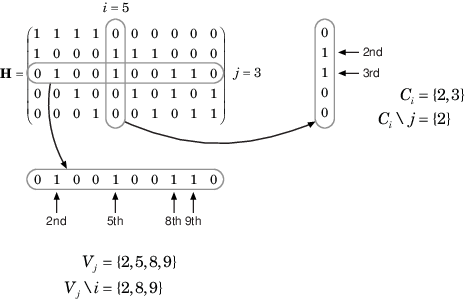
To avoid infinite numbers in the algorithm equations, atanh(1) and atanh(–1) are set to 19.07 and –19.07, respectively. Due to finite precision, MATLAB returns 1 for tanh(19.07) and –1 for tanh(-19.07).
Layered Belief Propagation Decoding. The implementation of the layered belief propagation algorithm is based on the decoding algorithm presented in Hocevar [3], Section II.A. The decoding loop iterates over subsets of rows (layers) of the PCM. For each row, m, in a layer and each bit index, j, the implementation updates the key components of the algorithm based on these equations:
(1) ,
(2) ,
(3) ,
(4) , and
(5) .
For each layer, the decoding equation (5) works on the combined input obtained from the current LLR inputs and the previous layer updates .
Because only a subset of the nodes is updated in a layer, the layered belief propagation algorithm is faster compared to the belief propagation algorithm. To achieve the same error rate as attained with belief propagation decoding, use half the number of decoding iterations when you use the layered belief propagation algorithm.
Normalized Min-Sum Decoding. The implementation of the normalized min-sum decoding algorithm follows the layered belief propagation algorithm with equation (2) replaced by
,
where α is in the range (0, 1] and is the scaling factor specified by the MinSumScalingFactor input argument to the ldpcDecode function. This equation is an adaptation of equation (4) presented in Chen [4].
Offset Min-Sum Decoding. The implementation of the offset min-sum decoding algorithm follows the layered belief propagation algorithm with equation (2) replaced by
,
where β ≥ 0 and is the offset specified by the MinSumOffset input argument to the ldpcDecode function. This equation is an adaptation of equation (5) presented in Chen [4].
Selected Bibliography for LDPC Coding
[1] IEEE® Std 802.11™-2020 (Revision of IEEE Std 802.11-2016). "Part 11: Wireless LAN Medium Access Control (MAC) and Physical Layer (PHY) Specifications." IEEE Standard for Information technology — Telecommunications and information exchange between systems. Local and metropolitan area networks — Specific requirements.
[2] Gallager, Robert G. Low-Density Parity-Check Codes. Cambridge, MA: MIT Press, 1963.
[3] Hocevar, D.E. "A reduced complexity decoder architecture via layered decoding of LDPC codes." In IEEE Workshop on Signal Processing Systems, 2004. SIPS 2004, 107-112. https://doi.org/10.1109/SIPS.2004.1363033.
[4] Chen, Jinghu, R.M. Tanner, C. Jones, and Yan Li. "Improved min-sum decoding algorithms for irregular LDPC codes." In Proceedings. International Symposium on Information Theory, 2005. ISIT 2005. https://doi.org/10.1109/ISIT.2005.1523374.