step
R2026bStep response of dynamic system
Syntax
Description
step computes the step response to a step change in input
value from U to U + dU after td time
units.
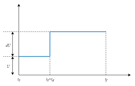
Here,
t0 is the simulation start time.
td is the step delay.
U is the baseline input value or bias.
dU is the step amplitude.
By default, the function applies step for t0 =
0, U = 0, dU = 1, and
td = 0. But, you can configure these values using
name-value arguments. You can also specify the initial state
x(t0). When you don't specify
the initial state, step assumes the system is initially at rest with
input level U.
[___] = step(___,
specifies response properties using one or more name-value arguments. For example,
Name=Value)step(sys,Bias=2) sets the input bias to 2. (since R2026b)
The following name-value arguments override values specified in other input arguments.
step(___) plots the step response of
sys with default plotting options for all of the previous input
argument combinations. For more plot customization options, use stepplot.
To plot responses for multiple dynamic systems on the same plot, you can specify
sysas a comma-separated list of models. For example,step(sys1,sys2,sys3)plots the responses for three models on the same plot.To specify a color, line style, and marker for each system in the plot, specify a
LineSpecvalue for each system. For example,step(sys1,LineSpec1,sys2,LineSpec2)plots two models and specifies their plot style. For more information on specifying aLineSpecvalue, seestepplot.
Examples
Plot the step response of a continuous-time system represented by the following transfer function.
For this example, create a tf model that represents the transfer function. You can similarly plot the step response of other dynamic system model types, such as zero-pole gain (zpk) or state-space (ss) models.
sys = tf(4,[1 2 10]);
Plot the step response.
step(sys)
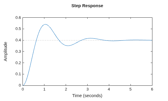
The step plot automatically includes a dotted horizontal line indicating the steady-state response. In a MATLAB® figure window, you can right-click the plot to view other step-response characteristics such as peak response and settling time. For more information about these characteristics, see stepinfo.
Plot the step response of a discrete-time system. The system has a sample time of 0.2 s and is represented by the following state-space matrices.
A = [1.6 -0.7;
      1  0];
B = [0.5; 0];
C = [0.1 0.1];
D = 0;
Create the state-space model and plot its step response.
sys = ss(A,B,C,D,0.2);
step(sys)
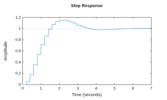
The step response reflects the discretization of the model, showing the response computed every 0.2 seconds.
Examine the step response of the following transfer function.
sys = zpk(-1,[-0.2+3j,-0.2-3j],1) * tf([1 1],[1 0.05])
sys =
            (s+1)^2
  ----------------------------
  (s+0.05) (s^2 + 0.4s + 9.04)

Continuous-time zero/pole/gain model.
Model Properties
step(sys)
By default, step chooses an end time that shows the steady state that the response is trending toward. This system has fast transients, however, which are obscured on this time scale. To get a closer look at the transient response, limit the step plot to t = 15 s.
step(sys,15)
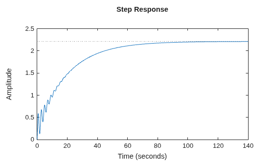
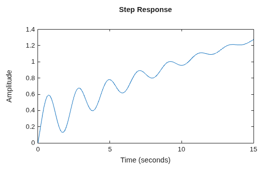
Alternatively, you can specify the exact times at which you want to examine the step response, provided they are separated by a constant interval. For instance, examine the response from the end of the transient until the system reaches steady state.
t = 20:0.2:120;
step(sys,t)
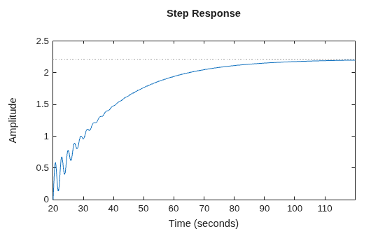
Even though this plot begins at t = 20, step always applies the step input at t = 0.
Consider the following second-order state-space model:
A = [-0.5572,-0.7814;0.7814,0];
B = [1,-1;0,2];
C = [1.9691,6.4493];
sys = ss(A,B,C,0);
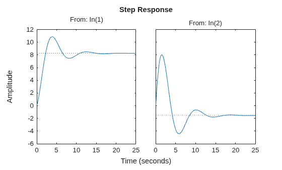
This model has two inputs and one output, so it has two channels: from the first input to the output, and from the second input to the output. Each channel has its own step response.
When you use step, it computes the responses of all channels.
step(sys)
The left plot shows the step response of the first input channel, and the right plot shows the step response of the second input channel. Whenever you use step to plot the responses of a MIMO model, it generates an array of plots representing all the I/O channels of the model. For instance, create a random state-space model with five states, three inputs, and two outputs, and plot its step response.
sys = rss(5,2,3);
step(sys)
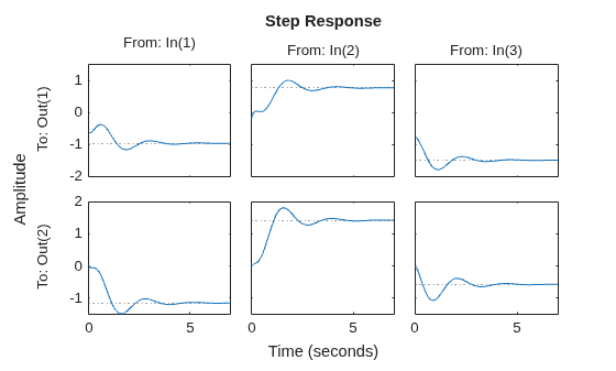
In a MATLAB figure window, you can restrict the plot to a subset of channels by right-clicking on the plot and selecting I/O Selector.
step allows you to plot the responses of multiple dynamic systems on the same axis. For instance, compare the closed-loop response of a system with a PI controller and a PID controller. Create a transfer function of the system and tune the controllers.
H = tf(4,[1 2 10]);
C1 = pidtune(H,'PI');
C2 = pidtune(H,'PID');
Form the closed-loop systems and plot their step responses.
sys1 = feedback(H*C1,1);
sys2 = feedback(H*C2,1);
step(sys1,sys2)
legend('PI','PID','Location','SouthEast')
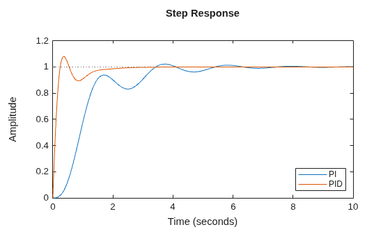
By default, step chooses distinct colors for each system that you plot. You can specify colors and line styles using the LineSpec input argument.
 step(sys1,'r--',sys2,'b')
 legend('PI','PID','Location','SouthEast')
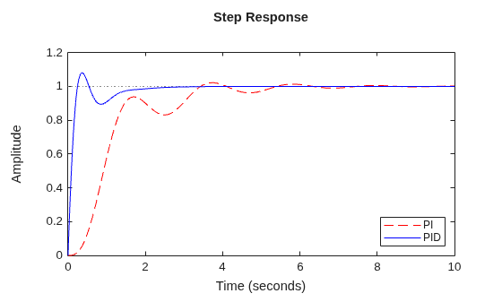
The first LineSpec 'r--' specifies a dashed red line for the response with the PI controller. The second LineSpec 'b' specifies a solid blue line for the response with the PID controller. The legend reflects the specified colors and linestyles. For more plot customization options, use stepplot.
The example Compare Responses of Multiple Systems shows how to plot responses of several individual systems on a single axis. When you have multiple dynamic systems arranged in a model array, step plots all their responses at once.
Create a model array. For this example, use a one-dimensional array of second-order transfer functions having different natural frequencies. First, preallocate memory for the model array. The following command creates a 1-by-5 row of zero-gain SISO transfer functions. The first two dimensions represent the model outputs and inputs. The remaining dimensions are the array dimensions.
sys = tf(zeros(1,1,1,5));
Populate the array.
w0 = 1.5:1:5.5;    % natural frequencies
zeta = 0.5;        % damping constant
for i = 1:length(w0)
   sys(:,:,1,i) = tf(w0(i)^2,[1 2*zeta*w0(i) w0(i)^2]);
end
(For more information about model arrays and how to create them, see Model Arrays.) Plot the step responses of all models in the array.
step(sys)
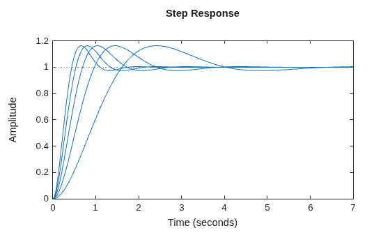
step uses the same linestyle for the responses of all entries in the array. One way to distinguish among entries is to use the SamplingGrid property of dynamic system models to associate each entry in the array with the corresponding w0 value.
sys.SamplingGrid = struct('frequency',w0);Now, when you plot the responses in a MATLAB figure window, you can click a trace to see which frequency value it corresponds to.
When you give it an output argument, step returns an array of response data. For a SISO system, the response data is returned as a column vector of length equal to the number of time points at which the response is sampled. You can provide the vector t of time points, or allow step to select time points for you based on system dynamics. For instance, extract the step response of a SISO system at 101 time points between t = 0 and t = 5 s.
sys = tf(4,[1 2 10]);
t = 0:0.05:5;
y = step(sys,t);
size(y)
ans = 1×2

   101     1
For a MIMO system, the response data is returned in an array of dimensions N-by-Ny-by-Nu, where Ny and Nu are the number of outputs and inputs of the dynamic system. For instance, consider the following state-space model, representing a two-input, one-output system.
A = [-0.5572,-0.7814;0.7814,0];
B = [1,-1;0,2];
C = [1.9691,6.4493];
sys = ss(A,B,C,0);
Extract the step response of this system at 200 time points between t = 0 and t = 20 s.
t = linspace(0,20,200);
y = step(sys,t);
size(y)
ans = 1×3

   200     1     2
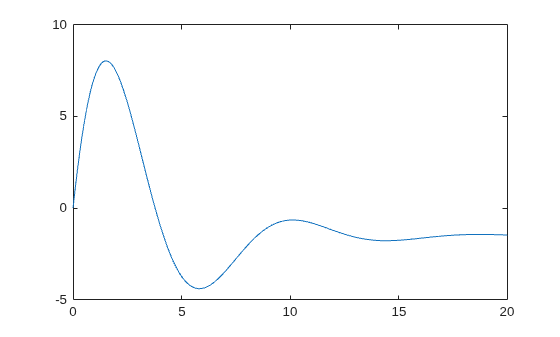
y(:,i,j) is a column vector containing the step response from the jth input to the ith output at the times t. For instance, extract the step response from the second input to the output.
y12 = y(:,1,2);
plot(t,y12)
Create a feedback loop with delay and plot its step response.
s = tf("s");
G = exp(-s) * (0.8*s^2+s+2)/(s^2+s);
sys = feedback(ss(G),1);
stepplot(sys)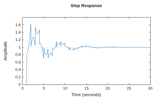
The system step response displayed is chaotic. The step response of systems with internal delays may exhibit odd behavior, such as recurring jumps. Such behavior is a feature of the system and not software anomalies.
By default, step applies an input signal that changes from 0 to 1 at t = 0. To customize the amplitude and bias, use name-value arguments. For instance, compute the response of a SISO state-space model to a signal that changes from 1 to –1 to at t = 0.
A = [1.6 -0.7;
      1  0];
B = [0.5; 0];
C = [0.1 0.1];
D = 0;
sys = ss(A,B,C,D,0.2);

step(sys, ...
    Bias=1, ...
    Amplitude= -2);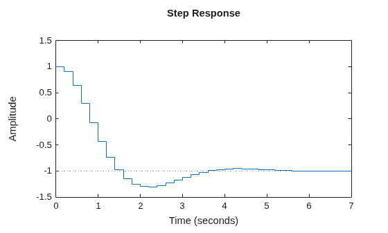
For responses to arbitrary input signals, use lsim.
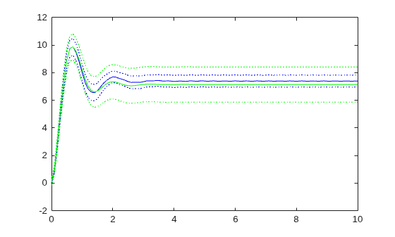
Compare the step response of a parametric identified model to a non-parametric (empirical) model. Also view their 3 confidence regions.
Load the data.
load iddata1 z1
Estimate a parametric model.
sys1 = ssest(z1,4);
Estimate a non-parametric model.
sys2 = impulseest(z1);
Plot the step responses for comparison.
t = (0:0.1:10)';
[y1, ~, ~, ysd1] = step(sys1,t);
[y2, ~, ~, ysd2] = step(sys2,t);
plot(t, y1, 'b', t, y1+3*ysd1, 'b:', t, y1-3*ysd1, 'b:')
hold on
plot(t, y2, 'g', t, y2+3*ysd2, 'g:', t, y2-3*ysd2, 'g:')
Compute the step response of an identified time-series model.
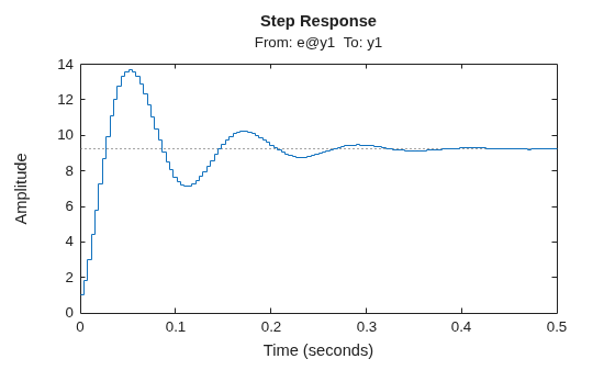
A time-series model, also called a signal model, is one without measured input signals. The step plot of this model uses its (unmeasured) noise channel as the input channel to which the step signal is applied.
Load the data.
load iddata9;Estimate a time-series model.
sys = ar(z9, 4);
sys is a model of the form A y(t) = e(t), where e(t) represents the noise channel. For computation of step response, e(t) is treated as an input channel, and is named e@y1.
Plot the step response.
step(sys)
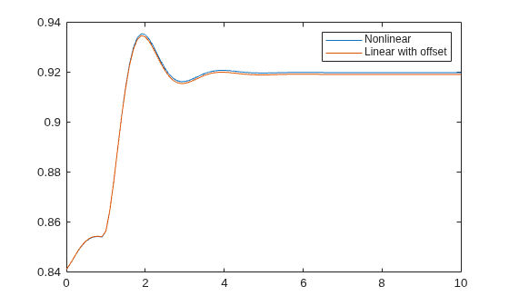
Validate the linearization of a nonlinear ARX model by comparing the small amplitude step responses of the linear and nonlinear models.
Load the data.
load iddata2 z2;
Estimate a nonlinear ARX model.
nlsys = nlarx(z2,[4 3 10],idTreePartition,"custom",...
    ["sin(y1(t-2)*u1(t))+y1(t-2)*u1(t)+u1(t).*u1(t-13)",...
    "y1(t-5)*y1(t-5)*y1(t-1)"],"nlr",[1:5, 7 9]);
Determine an equilibrium operating point for nlsys corresponding to a steady-state input value of 1.
u0 = 1;
[X,~,r] = findop(nlsys,"steady",1);
y0 = r.SignalLevels.Output;
Obtain a linear approximation of nlsys at this operating point.
sys = linearize(nlsys,u0,X);
Validate the usefulness of sys by comparing its small-amplitude step response to that of nlsys.
The nonlinear system nlsys is operating at an equilibrium level dictated by (u0,y0). Introduce a step perturbation of size 0.1 about this steady-state and compute the corresponding response.
t = (0:0.1:10)';
ynl = step(nlsys,t, ...
    Bias=u0, ...
    Amplitude=0.1);
The linear system sys expresses the relationship between the perturbations in input to the corresponding perturbation in output. It is unaware of the nonlinear system's equilibrium values.
Plot the step response of the linear system.
yl = step(sys,t, ...
    Amplitude=0.1);
Add the steady-state offset, y0, to the response of the linear system and plot the responses.
plot(t,ynl,t,yl+y0)
legend("Nonlinear","Linear with offset")
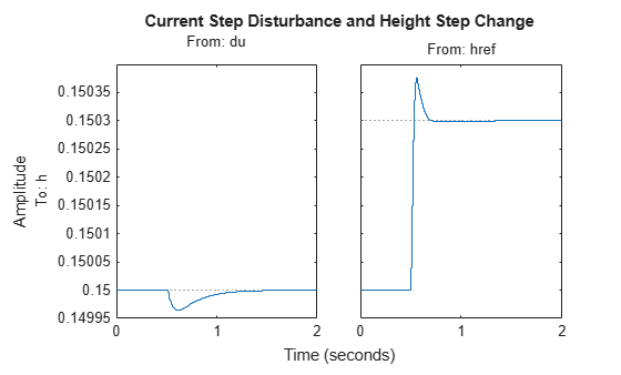
Compute and plot the step response of an LPV (lpvss) model. This example simulates the closed-loop step response of a levitating ball model defined in fcnMaglev.m to a disturbance .
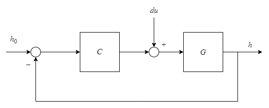
Create the model and discretize it.
hmin = 0.05;
hmax = 0.25;
h0 = (hmin+hmax)/2;
Ts = 0.01;
Glpv = lpvss("h",@fcnMaglev,0,0,h0);
Glpvd = c2d(Glpv,Ts,"tustin");
Sample the LPV model for three height values and tune a PID controller.
hpid = linspace(hmin,hmax,3);
[Ga,Goffset] = sample(Glpvd,[],hpid);
wc = 50;
Ka = pidtune(Ga,"pidf",wc);
Ka.Tf = 0.01;
Create the gain-scheduled PID controller.
Ka.SamplingGrid = struct("h",hpid);
Koffset = struct("y",{Goffset.u});
Clpv = ssInterpolant(ss(Ka),Koffset);
Create the closed-loop model.
CL = feedback(Glpvd*[1,Clpv],1,2,1);
CL.InputName = {'du';'href'};
CL.OutputName = "h";
Get steady-state current for = to compute an appropriate size for the step disturbance at the plant input.
[~,~,~,~,~,~,~,u0] = Glpv.DataFunction(0,h0);
Compute and plot the response to the input disturbance and step change in reference. Set the baseline input signals = 0 and = to specify the starting steady-state condition.
t = 0:Ts:2;
pFcn = @(k,x,u) x(1);
IC = findop(CL,t(1),h0,u=[u0;h0]);
stepplot(CL,t,pFcn, ...
    Amplitude=0.2*[u0;h0]*Ts, ...
    Delay=0.5, ...
    InitialCondition=IC)
title("Current Step Disturbance and Height Step Change")
Create a state-space model with complex coefficients.
A = [-2-2i -2;1 0];
B = [2;0];
C = [0 0.5+2.5i];
D = 0;
sys = ss(A,B,C,D);
Compute the step response of the system.
[y,t] = step(sys);
The resulting response data contains complex output values.
y
Since R2026a
This example shows why validation by varying sample time is necessary when simulating models with internal delays.
Load the model.
load idelayModel.mat
sys.InternalDelay
ans = 0.5166
Find the stability margins of sys. allmargin indicates that the closed-loop response should be unstable.
s = allmargin(sys)
s = struct with fields:
     GainMargin: [1.3867 0.9727 10.6798 20.1934 29.4912 38.7266 47.9352 57.1304 66.3172 75.4988 84.6770 93.8527 103.0266 112.1991 121.3705 130.5412 139.7111 148.8805 158.0495 167.2181 176.3864 185.5544 194.7221 203.8897 213.0571 222.2243 … ] (1×49 double)
    GMFrequency: [0.0467 5.0880 15.2373 27.3818 39.5403 51.7014 63.8635 76.0266 88.1895 100.3526 112.5158 124.6791 136.8424 149.0058 161.1692 173.3326 185.4960 197.6594 209.8229 221.9864 234.1499 246.3134 258.4768 270.6404 282.8039 … ] (1×49 double)
    PhaseMargin: [36.6926 -142.9664 113.4224 37.7140 -6.4674]
    PMFrequency: [0.0250 0.2899 0.8836 4.8597 5.1320]
    DelayMargin: [25.6083 13.0665 2.2403 0.1354 -0.0220]
    DMFrequency: [0.0250 0.2899 0.8836 4.8597 5.1320]
         Stable: 0
When you simulate the closed-loop response with the default step size, the response appears stable.
cl = feedback(sys,1);
figure
step(cl)
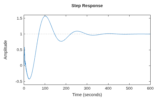
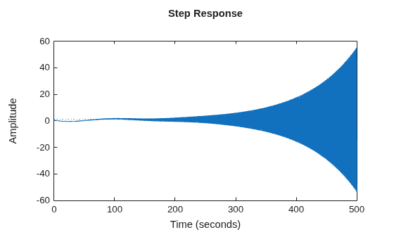
However, when you reduce the step size, the response reveals instability.
figure
step(cl,0:1e-2:500)
To gauge whether the selected time step size is small enough, you can compare the frequency response of the continuous and the discretized models with varying step size.
sysd1_cl = c2d(cl,0.4,'zoh');Warning: Discretization is only approximate due to internal delays. Use faster sampling rate if discretization error is large.
sysd2_cl = c2d(cl,0.01,'zoh');Warning: Discretization is only approximate due to internal delays. Use faster sampling rate if discretization error is large.
figure
bodeplot(cl,sysd1_cl,sysd2_cl)
legend("Continuous","Discrete (Ts = 0.4)","Discrete (Ts = 0.01)")
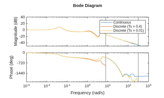
Slower sampling fails to fully capture resonance. Simulating models with internal delays is based on approximate discretization, so you must validate whether the selected step size is small enough by comparing the continuous and discrete responses in frequency domain.
Input Arguments
Name-Value Arguments
Output Arguments
Tips
To simulate system responses to arbitrary input signals, use
lsim.When you need additional plot customization options, use
stepplotinstead.Plots created using
stepdo not support multiline titles or labels specified as string arrays or cell arrays of character vectors. To specify multiline titles and labels, use a single string with anewlinecharacter.step(sys,u,t) title("first line" + newline + "second line");
Algorithms
To obtain samples of continuous-time models without internal delays,
step converts such models to state-space models and discretizes them
using a zero-order hold on the inputs. step chooses the sampling time for
this discretization automatically based on the system dynamics, except when you supply the
input time vector t in the form t = T0:dt:Tf. In that
case, step uses dt as the sampling time. The resulting
simulation time steps tOut are equisampled with spacing
dt.
For systems with internal delays, Control System Toolbox™ software uses simulations based on approximate c2d
discretization. The accuracy of simulation improves as sampling time decreases. For an
example, see Validate Simulation Results for Models with Internal Delays. (since R2026a)
References
[1] L.F. Shampine and P. Gahinet, "Delay-differential-algebraic equations in control theory," Applied Numerical Mathematics, Vol. 56, Issues 3–4, pp. 574–588.

