Creating Continuous-Time Models

LTI Model Types

Control System Toolbox™ provides functions for creating four basic representations of linear time-invariant (LTI) models:

These functions take model data as input and create objects that embody this data in a single MATLAB® variable.

Creating Transfer Function Models

Transfer functions (TF) are frequency-domain representations of LTI systems. A SISO transfer function is a ratio of polynomials:

Transfer functions are specified by their numerator and denominator polynomials A(s) and B(s). In MATLAB, a polynomial is represented by the vector of its coefficients, for example, the polynomial

is specified as [1 2 10].

To create a TF object representing the transfer function:

specify the numerator and denominator polynomials and use tf to construct the TF object:

num = [ 1  0 ];       % Numerator: s
den = [ 1  2  10 ];   % Denominator: s^2 + 2 s + 10
H = tf(num,den)

H =
 
        s
  --------------
  s^2 + 2 s + 10
 
Continuous-time transfer function.

Alternatively, you can specify this model as a rational expression of the Laplace variable s:

s = tf('s');        % Create Laplace variable
H = s / (s^2 + 2*s + 10)

H =
 
        s
  --------------
  s^2 + 2 s + 10
 
Continuous-time transfer function.

Creating Zero-Pole-Gain Models

Zero-pole-gain (ZPK) models are the factored form of transfer functions:

Such models expose the roots z of the numerator (the zeros) and the roots p of the denominator (the poles). The scalar coefficient k is called the gain.

To create the ZPK model:

specify the vectors of poles and zeros and the gain k:

z = 0;                   % Zeros
p = [ 2  1+i  1-i ];     % Poles
k = -2;                  % Gain
H = zpk(z,p,k)

H =
 
          -2 s
  --------------------
  (s-2) (s^2 - 2s + 2)
 
Continuous-time zero/pole/gain model.

As for TF models, you can also specify this model as a rational expression of s:

s = zpk('s');
H = -2*s / (s - 2) / (s^2 - 2*s + 2)

H =
 
          -2 s
  --------------------
  (s-2) (s^2 - 2s + 2)
 
Continuous-time zero/pole/gain model.

Creating State-Space Models

State-space (SS) models are time-domain representations of LTI systems:

where x(t) is the state vector, u(t) is input vector, and y(t) is the output trajectory.

State-space models are derived from the differential equations describing the system dynamics. For example, consider the second-order ODE for a simple electric motor:

where I is the driving current (input) and theta is the angular displacement of the rotor (output). This ODE can be rewritten in state-space form as:

To create this model, specify the state-space matrices A, B, C, D and use ss to construct the SS object:

A = [ 0  1 ; -5  -2 ];
B = [ 0 ; 3 ];
C = [ 1  0 ];
D = 0;
H = ss(A,B,C,D)

H =
 
  A = 
       x1  x2
   x1   0   1
   x2  -5  -2
 
  B = 
       u1
   x1   0
   x2   3
 
  C = 
       x1  x2
   y1   1   0
 
  D = 
       u1
   y1   0
 
Continuous-time state-space model.

Creating Frequency Response Data Models

Frequency response data (FRD) models let you store the measured or simulated complex frequency response of a system in an LTI object. You can then use this data as a surrogate model for frequency-domain analysis and design purposes.

For example, suppose you get the following data out of a frequency analyzer:

You can create an FRD object containing this data using:

freq = [10, 30, 50, 100, 500];
resp = [0.0021+0.0009i, 0.0027+0.0029i, 0.0044+0.0052i, 0.0200-0.0040i, 0.0001-0.0021i];
H = frd(resp,freq,'Units','Hz')

H =
 
    Frequency(Hz)           Response       
    -------------           --------       
          10         2.100e-03 + 9.000e-04i
          30         2.700e-03 + 2.900e-03i
          50         4.400e-03 + 5.200e-03i
         100         2.000e-02 - 4.000e-03i
         500         1.000e-04 - 2.100e-03i
 
Continuous-time frequency response.

Note that frequency values are assumed to be in rad/s unless you specify the Units to be Hertz.

Creating MIMO Models

The tf, zpk, ss, and frd commands let you construct both SISO and MIMO models. For TF or ZPK models, it is often convenient to construct MIMO models by concatenating simpler SISO models. For example, you can create the 2x2 MIMO transfer function:

using:

s = tf('s');
H = [ 1/(s+1) , 0 ; (s+1)/(s^2+s+3) , -4*s/(s+2) ]

H =
 
  From input 1 to output...
         1
   1:  -----
       s + 1
 
          s + 1
   2:  -----------
       s^2 + s + 3
 
  From input 2 to output...
   1:  0
 
       -4 s
   2:  -----
       s + 2
 
Continuous-time transfer function.

Analyzing LTI Models

Control System Toolbox provides an extensive set of functions for analyzing LTI models. These functions range from simple queries about I/O size and order to sophisticated time and frequency response analysis.

For example, you can obtain size information for the MIMO transfer function H specified above by typing:

size(H)

Transfer function with 2 outputs and 2 inputs.

You can compute the poles using:

pole(H)

ans = 4×1 complex

  -1.0000 + 0.0000i
  -0.5000 + 1.6583i
  -0.5000 - 1.6583i
  -2.0000 + 0.0000i

You can ask whether this system is stable using:

isstable(H)

ans = logical
   1

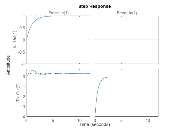
Finally, you can plot the step response by typing:

step(H)