Vehicle Detection Using ResNet-18 Based YOLO v2 Deployed to FPGA
This example shows how to train and deploy a you only look once (YOLO) v2 object detector.
Deep learning is a powerful machine learning technique that you can use to train robust object detectors. Several techniques for object detection exist, including Faster R-CNN and you only look once (YOLO) v2. This example trains a YOLO v2 vehicle detector using the trainYOLOv2ObjectDetector function.
Load Dataset
This example uses a small vehicle dataset that contains 295 images. Many of these images come from the Caltech Cars 1999 and 2001 data sets, available at the Caltech Computational Vision website, created by Pietro Perona and used with permission. Each image contains one or two labeled instances of a vehicle. A small dataset is useful for exploring the YOLO v2 training procedure, but in practice, more labeled images are needed to train a robust detector. The data set is attached to the example. Unzip the vehicle images and load the vehicle ground truth data.
unzip vehicleDatasetImages.zip
data = load('vehicleDatasetGroundTruth.mat');
vehicleDataset = data.vehicleDataset;
The vehicle data is stored in a two-column table, where the first column contains the image file paths and the second column contains the vehicle bounding boxes.
% Add the fullpath to the local vehicle data folder.
vehicleDataset.imageFilename = fullfile(pwd,vehicleDataset.imageFilename);
Split the dataset into training and test sets. Select 60% of the data for training and the rest for testing the trained detector.
rng(0);
shuffledIndices = randperm(height(vehicleDataset));
idx = floor(0.6 * length(shuffledIndices) );
trainingDataTbl = vehicleDataset(shuffledIndices(1:idx),:);
testDataTbl = vehicleDataset(shuffledIndices(idx+1:end),:);
Use imageDatastore and boxLabelDataStore to create datastores for loading the image and label data during training and evaluation.
imdsTrain = imageDatastore(trainingDataTbl{:,'imageFilename'});
bldsTrain = boxLabelDatastore(trainingDataTbl(:,'vehicle'));

imdsTest = imageDatastore(testDataTbl{:,'imageFilename'});
bldsTest = boxLabelDatastore(testDataTbl(:,'vehicle'));
Combine image and box label datastores.
trainingData = combine(imdsTrain,bldsTrain);
testData = combine(imdsTest,bldsTest);
Create a YOLO v2 Object Detection Network
A YOLO v2 object detection network is composed of two subnetworks. A feature extraction network followed by a detection network. The feature extraction network is typically a pretrained CNN (for details, see Pretrained Deep Neural Networks). This example uses ResNet-18 for feature extraction. You can also use other pretrained networks such as MobileNet v2 or ResNet-50 depending on application requirements. The detection sub-network is a small CNN compared to the feature extraction network and is composed of a few convolutional layers and layers specific for YOLO v2.
First, specify the network input size. When choosing the network input size, consider the minimum size required by the network itself, the size of the training images, and the computational cost incurred by processing data at the selected size. When feasible, choose a network input size that is close to the size of the training image and larger than the input size required for the network. To reduce the computational cost of running the example, specify a network input size of [224 224 3], which is the minimum size required to run the network.
inputSize = [224 224 3];
Define the names of object classes to detect.
className = "vehicle";Estimate Anchor Boxes
Note that the training images used in this example vary in size and are bigger than the network input size, 224-by-224. To correct this, resize the images in a preprocessing step prior to training.
Next, use estimateAnchorBoxes (Computer Vision Toolbox) to estimate anchor boxes based on the size of objects in the training data. To account for the resizing of the images prior to training, resize the training data for estimating anchor boxes. Use transform to preprocess the training data, then define the number of anchor boxes and estimate the anchor boxes. Resize the training data to the input image size of the network using the supporting function yolo_preprocessData.
trainingDataForEstimation = transform(trainingData,@(data)yolo_preprocessData(data,inputSize));
numAnchors = 7;
[anchorBoxes, meanIoU] = estimateAnchorBoxes(trainingDataForEstimation,numAnchors)
anchorBoxes = 7×2

     40     38
    156    127
     74     71
    135    121
     36     25
     56     52
     98     89
meanIoU =
0.8383
For more information on choosing anchor boxes, see Estimate Anchor Boxes from Training Data (Computer Vision Toolbox) and Anchor Boxes for Object Detection (Computer Vision Toolbox).
Now, use imagePretrainedNetwork to load a pretrained ResNet-18 model.
baseNet = imagePretrainedNetwork("resnet18");Select 'res4b_relu' as the feature extraction layer to replace the layers after 'res4b_relu' with the detection subnetwork. This feature extraction layer outputs feature maps that are downsampled by a factor of 16. This amount of downsampling is a good trade-off between spatial resolution and the strength of the extracted features, as features extracted further down the network encode stronger image features at the cost of spatial resolution. Choosing the optimal feature extraction layer requires empirical analysis.
featureExtractionLayer = 'res4b_relu';Create a YOLO v2 object detection network.
detector = yolov2ObjectDetector(baseNet,className,anchorBoxes,DetectionNetworkSource=featureExtractionLayer);
You can visualize the network using analyzeNetwork or Deep Network Designer from Deep Learning Toolbox™.
Data Augmentation
Data augmentation is used to improve network accuracy by randomly transforming the original data during training. By using data augmentation you can add more variety to the training data without actually having to increase the number of labeled training samples.
Use transform to augment the training data by randomly flipping the image and associated box labels horizontally. Note that data augmentation is not applied to the test and validation data. Ideally, test and validation data should be representative of the original data and is left unmodified for unbiased evaluation.
augmentedTrainingData = transform(trainingData,@yolo_augmentData);
Preprocess Training Data and Train YOLO v2 Object Detector
Preprocess the augmented training data, and the validation data to prepare for training.
preprocessedTrainingData = transform(augmentedTrainingData,@(data)yolo_preprocessData(data,inputSize));
Use trainingOptions to specify network training options. Set 'ValidationData' to the preprocessed validation data. Set 'CheckpointPath' to a temporary location. This enables the saving of partially trained detectors during the training process. If training is interrupted, such as by a power outage or system failure, you can resume training from the saved checkpoint.
options = trainingOptions('sgdm', ...
        'MiniBatchSize', 16, ....
        'InitialLearnRate',1e-3, ...
        'MaxEpochs',20,...
        'CheckpointPath', tempdir, ...
        'Shuffle','never');
Use trainYOLOv2ObjectDetector (Computer Vision Toolbox) function to train YOLO v2 object detector.
[detector,info] = trainYOLOv2ObjectDetector(preprocessedTrainingData,detector,options);
*************************************************************************
Training a YOLO v2 Object Detector for the following object classes:

* vehicle

Training on single GPU.
|========================================================================================|
|  Epoch  |  Iteration  |  Time Elapsed  |  Mini-batch  |  Mini-batch  |  Base Learning  |
|         |             |   (hh:mm:ss)   |     RMSE     |     Loss     |      Rate       |
|========================================================================================|
|       1 |           1 |       00:00:01 |         8.34 |         69.6 |          0.0010 |
|       5 |          50 |       00:00:29 |         0.80 |          0.6 |          0.0010 |
|      10 |         100 |       00:00:58 |         0.72 |          0.5 |          0.0010 |
|      14 |         150 |       00:01:24 |         0.55 |          0.3 |          0.0010 |
|      19 |         200 |       00:01:51 |         0.53 |          0.3 |          0.0010 |
|      20 |         220 |       00:01:59 |         0.54 |          0.3 |          0.0010 |
|========================================================================================|
Training finished: Max epochs completed.
Detector training complete.
*************************************************************************
As a quick test, run the detector on one test image. Make sure you resize the image to the same size as the training images.
% Read the datastore.
data = read(testData);

% Get the image.
I = data{1};
I = imresize(I,inputSize(1:2));
[bboxes,scores] = detect(detector,I);
Display the results.
I_new = insertObjectAnnotation(I,'rectangle',bboxes,scores);
figure
imshow(I_new)
Load Pretrained Network
Load the pretrained network.
net = detector.Network;
I_pre=yolo_pre_proc(I);
Use deepNetworkDesigner to obtain information about the network layers:
deepNetworkDesigner(net)
Create Target Object
Create a target object for your target device with a vendor name and an interface to connect your target device to the host computer. Interface options are JTAG (default) and Ethernet. Vendor options are Intel or Xilinx®. Use the installed Xilinx Vivado® Design Suite over an Ethernet connection to program the device.
hTarget = dlhdl.Target('Xilinx', 'Interface', 'Ethernet');
Create Workflow Object
Create an object of the dlhdl.Workflow class. When you create the object, specify the network and the bitstream name. Specify the saved pre-trained series network, trainedNetNoCar, as the network. Make sure the bitstream name matches the data type and the FPGA board that you are targeting. In this example, the target FPGA board is the Zynq® UltraScale™+ MPSoC ZCU102 board. The bitstream uses single data type.
hW=dlhdl.Workflow('Network', net, 'Bitstream', 'zcu102_single','Target',hTarget)
hW =
  Workflow with properties:

      Network: [1×1 dlnetwork]
    Bitstream: [1×1 dnnfpga.bitstream.Bitstream]
       Target: [1×1 dnnfpga.hardware.TargetEthernet]
Compile YOLO v2 Object Detector
To compile the network net, run the compile function of the dlhdl.Workflow object.
dn = hW.compile
### Compiling network for Deep Learning FPGA prototyping ...
### Targeting FPGA bitstream zcu102_single.
### An output layer called 'Output1_yolov2Transform' of type 'nnet.cnn.layer.RegressionOutputLayer' has been added to the provided network. This layer performs no operation during prediction and thus does not affect the output of the network.
### Optimizing network: Fused 'nnet.cnn.layer.BatchNormalizationLayer' into 'nnet.cnn.layer.Convolution2DLayer'
### The network includes the following layers:
     1   'data'                      Image Input               224×224×3 images                                                      (SW Layer)
     2   'conv1'                     2-D Convolution           64 7×7×3 convolutions with stride [2  2] and padding [3  3  3  3]     (HW Layer)
     3   'conv1_relu'                ReLU                      ReLU                                                                  (HW Layer)
     4   'pool1'                     2-D Max Pooling           3×3 max pooling with stride [2  2] and padding [1  1  1  1]           (HW Layer)
     5   'res2a_branch2a'            2-D Convolution           64 3×3×64 convolutions with stride [1  1] and padding [1  1  1  1]    (HW Layer)
     6   'res2a_branch2a_relu'       ReLU                      ReLU                                                                  (HW Layer)
     7   'res2a_branch2b'            2-D Convolution           64 3×3×64 convolutions with stride [1  1] and padding [1  1  1  1]    (HW Layer)
     8   'res2a'                     Addition                  Element-wise addition of 2 inputs                                     (HW Layer)
     9   'res2a_relu'                ReLU                      ReLU                                                                  (HW Layer)
    10   'res2b_branch2a'            2-D Convolution           64 3×3×64 convolutions with stride [1  1] and padding [1  1  1  1]    (HW Layer)
    11   'res2b_branch2a_relu'       ReLU                      ReLU                                                                  (HW Layer)
    12   'res2b_branch2b'            2-D Convolution           64 3×3×64 convolutions with stride [1  1] and padding [1  1  1  1]    (HW Layer)
    13   'res2b'                     Addition                  Element-wise addition of 2 inputs                                     (HW Layer)
    14   'res2b_relu'                ReLU                      ReLU                                                                  (HW Layer)
    15   'res3a_branch2a'            2-D Convolution           128 3×3×64 convolutions with stride [2  2] and padding [1  1  1  1]   (HW Layer)
    16   'res3a_branch2a_relu'       ReLU                      ReLU                                                                  (HW Layer)
    17   'res3a_branch2b'            2-D Convolution           128 3×3×128 convolutions with stride [1  1] and padding [1  1  1  1]  (HW Layer)
    18   'res3a_branch1'             2-D Convolution           128 1×1×64 convolutions with stride [2  2] and padding [0  0  0  0]   (HW Layer)
    19   'res3a'                     Addition                  Element-wise addition of 2 inputs                                     (HW Layer)
    20   'res3a_relu'                ReLU                      ReLU                                                                  (HW Layer)
    21   'res3b_branch2a'            2-D Convolution           128 3×3×128 convolutions with stride [1  1] and padding [1  1  1  1]  (HW Layer)
    22   'res3b_branch2a_relu'       ReLU                      ReLU                                                                  (HW Layer)
    23   'res3b_branch2b'            2-D Convolution           128 3×3×128 convolutions with stride [1  1] and padding [1  1  1  1]  (HW Layer)
    24   'res3b'                     Addition                  Element-wise addition of 2 inputs                                     (HW Layer)
    25   'res3b_relu'                ReLU                      ReLU                                                                  (HW Layer)
    26   'res4a_branch2a'            2-D Convolution           256 3×3×128 convolutions with stride [2  2] and padding [1  1  1  1]  (HW Layer)
    27   'res4a_branch2a_relu'       ReLU                      ReLU                                                                  (HW Layer)
    28   'res4a_branch2b'            2-D Convolution           256 3×3×256 convolutions with stride [1  1] and padding [1  1  1  1]  (HW Layer)
    29   'res4a_branch1'             2-D Convolution           256 1×1×128 convolutions with stride [2  2] and padding [0  0  0  0]  (HW Layer)
    30   'res4a'                     Addition                  Element-wise addition of 2 inputs                                     (HW Layer)
    31   'res4a_relu'                ReLU                      ReLU                                                                  (HW Layer)
    32   'res4b_branch2a'            2-D Convolution           256 3×3×256 convolutions with stride [1  1] and padding [1  1  1  1]  (HW Layer)
    33   'res4b_branch2a_relu'       ReLU                      ReLU                                                                  (HW Layer)
    34   'res4b_branch2b'            2-D Convolution           256 3×3×256 convolutions with stride [1  1] and padding [1  1  1  1]  (HW Layer)
    35   'res4b'                     Addition                  Element-wise addition of 2 inputs                                     (HW Layer)
    36   'res4b_relu'                ReLU                      ReLU                                                                  (HW Layer)
    37   'yolov2Conv1'               2-D Convolution           256 3×3×256 convolutions with stride [1  1] and padding 'same'        (HW Layer)
    38   'yolov2Relu1'               ReLU                      ReLU                                                                  (HW Layer)
    39   'yolov2Conv2'               2-D Convolution           256 3×3×256 convolutions with stride [1  1] and padding 'same'        (HW Layer)
    40   'yolov2Relu2'               ReLU                      ReLU                                                                  (HW Layer)
    41   'yolov2ClassConv'           2-D Convolution           42 1×1×256 convolutions with stride [1  1] and padding [0  0  0  0]   (HW Layer)
    42   'yolov2Transform'           YOLO v2 Transform Layer   YOLO v2 Transform Layer with 7 anchors                                (SW Layer)
    43   'Output1_yolov2Transform'   Regression Output         mean-squared-error                                                    (SW Layer)

### Notice: The layer 'data' with type 'nnet.cnn.layer.ImageInputLayer' is implemented in software.
### Notice: The layer 'yolov2Transform' with type 'nnet.cnn.layer.YOLOv2TransformLayer' is implemented in software.
### Notice: The layer 'Output1_yolov2Transform' with type 'nnet.cnn.layer.RegressionOutputLayer' is implemented in software.
### Compiling layer group: conv1>>pool1 ...
### Compiling layer group: conv1>>pool1 ... complete.
### Compiling layer group: res2a_branch2a>>res2a_branch2b ...
### Compiling layer group: res2a_branch2a>>res2a_branch2b ... complete.
### Compiling layer group: res2b_branch2a>>res2b_branch2b ...
### Compiling layer group: res2b_branch2a>>res2b_branch2b ... complete.
### Compiling layer group: res3a_branch1 ...
### Compiling layer group: res3a_branch1 ... complete.
### Compiling layer group: res3a_branch2a>>res3a_branch2b ...
### Compiling layer group: res3a_branch2a>>res3a_branch2b ... complete.
### Compiling layer group: res3b_branch2a>>res3b_branch2b ...
### Compiling layer group: res3b_branch2a>>res3b_branch2b ... complete.
### Compiling layer group: res4a_branch1 ...
### Compiling layer group: res4a_branch1 ... complete.
### Compiling layer group: res4a_branch2a>>res4a_branch2b ...
### Compiling layer group: res4a_branch2a>>res4a_branch2b ... complete.
### Compiling layer group: res4b_branch2a>>res4b_branch2b ...
### Compiling layer group: res4b_branch2a>>res4b_branch2b ... complete.
### Compiling layer group: yolov2Conv1>>yolov2ClassConv ...
### Compiling layer group: yolov2Conv1>>yolov2ClassConv ... complete.

### Allocating external memory buffers:

          offset_name          offset_address    allocated_space
    _______________________    ______________    ________________

    "InputDataOffset"           "0x00000000"     "23.0 MB"
    "OutputResultOffset"        "0x016f8000"     "1012.0 kB"
    "SchedulerDataOffset"       "0x017f5000"     "2.4 MB"
    "SystemBufferOffset"        "0x01a54000"     "6.2 MB"
    "InstructionDataOffset"     "0x02081000"     "2.1 MB"
    "ConvWeightDataOffset"      "0x0229d000"     "17.5 MB"
    "EndOffset"                 "0x0341a000"     "Total: 52.1 MB"

### Network compilation complete.
dn = struct with fields:
             weights: [1×1 struct]
        instructions: [1×1 struct]
           registers: [1×1 struct]
    syncInstructions: [1×1 struct]
        constantData: {}
             ddrInfo: [1×1 struct]
       resourceTable: [6×2 table]
Program the Bitstream onto FPGA and Download Network Weights
To deploy the network on the Zynq UltraScale+ MPSoC ZCU102 hardware, run the deploy function of the dlhdl.Workflow object. This function uses the output of the compile function to program the FPGA board by using the programming file.The function also downloads the network weights and biases. The deploy function checks for the Xilinx Vivado tool and the supported tool version. It then starts programming the FPGA device by using the bitstream, displays progress messages and the time it takes to deploy the network.
hW.deploy
### Programming FPGA Bitstream using Ethernet...
### Attempting to connect to the hardware board at 192.168.1.101...
### Connection successful
### Programming FPGA device on Xilinx SoC hardware board at 192.168.1.101...
### Attempting to connect to the hardware board at 192.168.1.101...
### Connection successful
### Copying FPGA programming files to SD card...
### Setting FPGA bitstream and devicetree for boot...
# Copying Bitstream zcu102_single.bit to /mnt/hdlcoder_rd
# Set Bitstream to hdlcoder_rd/zcu102_single.bit
# Copying Devicetree devicetree_dlhdl.dtb to /mnt/hdlcoder_rd
# Set Devicetree to hdlcoder_rd/devicetree_dlhdl.dtb
# Set up boot for Reference Design: 'AXI-Stream DDR Memory Access : 3-AXIM'
### Programming done. The system will now reboot for persistent changes to take effect.
### Rebooting Xilinx SoC at 192.168.1.101...
### Reboot may take several seconds...
### Attempting to connect to the hardware board at 192.168.1.101...
### Connection successful
### Programming the FPGA bitstream has been completed successfully.
### Loading weights to Conv Processor.
### Conv Weights loaded. Current time is 19-Jul-2024 11:26:12
Load the Example Image and Run the Prediction
Execute the predict function on the dlhdl.Workflow object and display the result:
I_pre_dlarray = dlarray(I_pre, 'SSCB');
[prediction, speed] = hW.predict(I_pre_dlarray,'Profile','on');
### Finished writing input activations.
### Running single input activation.


              Deep Learning Processor Profiler Performance Results

                   LastFrameLatency(cycles)   LastFrameLatency(seconds)       FramesNum      Total Latency     Frames/s
                         -------------             -------------              ---------        ---------       ---------
Network                   17389625                  0.07904                       1           17391542             12.6
    conv1                  2226697                  0.01012
    pool1                   505544                  0.00230
    res2a_branch2a          974406                  0.00443
    res2a_branch2b          974296                  0.00443
    res2a                   374032                  0.00170
    res2b_branch2a          974184                  0.00443
    res2b_branch2b          974139                  0.00443
    res2b                   373892                  0.00170
    res3a_branch1           539776                  0.00245
    res3a_branch2a          542191                  0.00246
    res3a_branch2b          909831                  0.00414
    res3a                   186935                  0.00085
    res3b_branch2a          909773                  0.00414
    res3b_branch2b          909981                  0.00414
    res3b                   187011                  0.00085
    res4a_branch1           491442                  0.00223
    res4a_branch2a          494901                  0.00225
    res4a_branch2b          894073                  0.00406
    res4a                    93584                  0.00043
    res4b_branch2a          894129                  0.00406
    res4b_branch2b          894092                  0.00406
    res4b                    93594                  0.00043
    yolov2Conv1             893960                  0.00406
    yolov2Conv2             894973                  0.00407
    yolov2ClassConv         182041                  0.00083
 * The clock frequency of the DL processor is: 220MHz
Display the prediction results.
prediction = extractdata(prediction);
[bboxesn, scoresn, labelsn] = yolo_post_proc(prediction,I_pre,anchorBoxes,{'Vehicle'});
I_new3 = insertObjectAnnotation(I,'rectangle',bboxesn,scoresn);
figure
imshow(I_new3)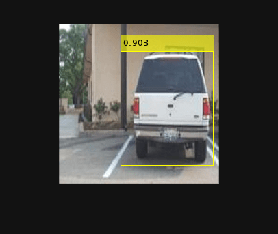
See Also
dlhdl.Workflow | dlhdl.Target | compile | deploy | predict | dlquantizer | dlquantizationOptions | calibrate | validate