Machine Learning and Deep Learning Classification Using Signal Feature Extraction Objects
This example uses signal feature extraction objects to extract multidomain features that you can use to identify faulty bearing signals in mechanical systems. Feature extraction objects enable you to efficiently compute multiple features by reducing the number of times that signals are transformed into a particular domain. All the feature extraction code is run using a CPU with a single worker. To learn how to extract features and train models in parallel using a parallel pool of workers, see Accelerate Signal Feature Extraction and Classification Using a Parallel Pool of Workers (Signal Processing Toolbox). To learn how to extract features and train models using a GPU, see Accelerate Signal Feature Extraction and Classification Using a GPU (Signal Processing Toolbox).
Rotating machines that use bearings are widely employed in industrial applications such as food processing, paper making, and manufacturing of medical devices, semiconductors, and aircraft components. Industrial systems used in these fields often suffer from electric current discharged through the bearings that can result in motor bearing failure within a few months of system startup. Failure to detect these issues in a timely manner can cause significant downtime in system operations. In addition to requiring regularly scheduled maintenance, the industrial system using rotating machines needs continuous monitoring for bearing current detection to ensure safety, reliability, efficiency, and performance.
Significant research has been dedicated to automatic identification of faulty bearings in industrial systems. Reliable, effective, and efficient feature extraction techniques play a key role in AI-based fault diagnosis performance [1], [2]. As the bearing current is caused by variable speed conditions, the fault frequencies can sweep up or down in the frequency range over time as the speed varies. In other words, bearing vibration signals are nonstationary in nature. The nonstationary characteristics can be captured well by various time-frequency representations. Combined features extracted from the time, frequency, and time-frequency representations of the signals can be used to improve the fault detection performance of systems [3].
Download and Prepare Data
The data set contains acceleration signals collected from rotating machines in a bearing test rig and from real-world machines such as oil pump bearings, intermediate speed bearings, and a planet bearing. There are 34 files in total. The signals in the files are sampled at fs = 48828 Hz. The filenames describe the signals they contain:
HealthySignal_*.mat—Healthy signalsInnerRaceFault_*.mat—Signals with inner race faultsOuterRaceFault_*.mat—Signals with outer race faults
Download the data files into temporary directory. Create a signalDatastore object to access the data in the files and obtain the labels denoting the signal category.
dataURL = "https://www.mathworks.com/supportfiles/SPT/data/rollingBearingDataset.zip";
datasetFolder = fullfile(tempdir,"rollingBearingDataset");
zipFile = fullfile(tempdir,"rollingBearingDataset.zip");
if ~exist(datasetFolder,"dir")
    websave(zipFile,dataURL);
    unzip(zipFile,datasetFolder);
end

sds = signalDatastore(datasetFolder);
Filenames in the data set includes the labels. Get a list of labels from the filenames in the datastore using the filenames2labels (Signal Processing Toolbox) function.
labels = filenames2labels(sds,ExtractBefore=pattern("Signal"|"Fault"));
Analyze one healthy signal, one signal with inner race faults, and one signal with outer race faults in using their spectrogram representation.
healthySignal = read(subset(sds,1));
innerRaceFaultSignal = read(subset(sds,13));
outerRaceFaultSignal = read(subset(sds,34));

fs = 48828;

figure
tiledlayout(3,2)
nexttile
plot((0:numel(healthySignal)-1)/fs,healthySignal)
xlabel("Time (seconds)")
title("Healthy")
nexttile
pspectrum(healthySignal,fs,"spectrogram",Leakage=0.9)
title("Healthy")

nexttile
plot((0:numel(innerRaceFaultSignal)-1)/fs,innerRaceFaultSignal)
xlabel("Time (seconds)")
title("Inner Race")
nexttile
pspectrum(innerRaceFaultSignal,fs,"spectrogram",Leakage=0.9)
title("Inner Race")

nexttile
plot((0:numel(outerRaceFaultSignal)-1)/fs,outerRaceFaultSignal)
xlabel("Time (seconds)")
title("Outer Race")
nexttile
pspectrum(outerRaceFaultSignal,fs,"spectrogram",Leakage=0.9)
title("Outer Race")
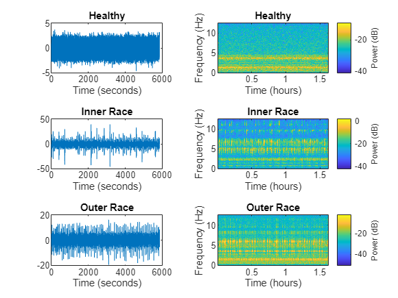
The spectrogram for the healthy signal shows that the frequency content over time is more concentrated in the low-frequency range. In contrast, the spectrograms for the faulty signals are spread out in both the low-frequency range and in the high-frequency range.
Set Up Feature Extraction Objects
Set up feature extraction objects that extract multidomain features from the signals. Then, use these features to implement machine learning and deep learning solutions to classify signals as healthy, as having inner race faults, or as having outer race faults.
Use the signalTimeFeatureExtractor, signalFrequencyFeatureExtractor, and signalTimeFrequencyFeatureExtractor objects to extract features from all the signals.
For time domain, use root-mean-square value, impulse factor, standard deviation, and clearance factor as features.
For frequency domain, use median frequency, band power, power bandwidth, and peak amplitude of the power spectral density (PSD) as features.
For time-frequency domain, use time-averaged wavelet spectrum as a feature.
Create a time-domain feature extractor to extract time-domain features.
timeFE = signalTimeFeatureExtractor(SampleRate=fs, ...
    RMS=true, ...
    ImpulseFactor=true, ...
    StandardDeviation=true, ...
    ClearanceFactor=true);
Create a frequency-domain feature extractor to extract frequency-domain features.
 freqFE = signalFrequencyFeatureExtractor(SampleRate=fs, ...
    MedianFrequency=true, ...
    BandPower=true, ...
    PowerBandwidth=true, ...
    PeakAmplitude=true);
Create a time-frequency feature extractor to extract time-frequency features from scalogram.
timeFreqFE = signalTimeFrequencyFeatureExtractor(SampleRate=fs, ...
    TimeSpectrum=true);

setExtractorParameters(timeFreqFE,"scalogram", ...
    VoicesPerOctave=16,FrequencyLimits=[50 20000]);
Train SVM Classifier Using Multidomain Features
Extract Multidomain Features
Extract features using all three features extractors for the signals in the signalDatastore object.
Concatenate the extracted features to obtain a feature matrix. You can use the feature matrix and its corresponding labels to train a multiclass SVM classifier.
SVMFeatures = cellfun(@(a,b,c) [a b c],extract(timeFE,sds), ...
    extract(freqFE,sds),extract(timeFreqFE,sds),UniformOutput=false);

featureMatrix = cell2mat(SVMFeatures);
Train SVM Classifier Model
Obtain a feature table from the multidomain feature matrix that you will use to train a multiclass SVM classifier and observe the classification accuracy.
featureTable = array2table(featureMatrix);

head(featureTable(:,1:6))
    featureMatrix1    featureMatrix2    featureMatrix3    featureMatrix4    featureMatrix5    featureMatrix6
    ______________    ______________    ______________    ______________    ______________    ______________

       0.89042           0.87979            7.7551            6.5588            6707.4           0.79563
       0.86631           0.86443            6.9682            5.9044            6744.8           0.74962
       0.87483           0.87293            7.2224            6.1184            6681.8           0.76698
       0.89696           0.89521            6.5476            5.5462            6632.1           0.80326
       0.88766           0.87685            7.2062            6.1101            6686.3           0.78838
       0.88632           0.87554            6.7042            5.6771            6724.6           0.78578
       0.89654           0.88599            6.8998            5.8484            6668.7            0.8064
       0.86256           0.85424            7.1177            6.0223              6845           0.74237
The feature table shows that the fifth feature of the table, which corresponds to the median frequency, is numerically much larger than the others and can thus dominate the learning process. To ensure that all the feature entries have the same weight in the training process, normalize the feature matrix.
Split the feature matrix into training and testing feature matrices. Obtain their corresponding labels. For reproducible results, reset the random seed generator.
rng("default")

cvp = cvpartition(labels,Holdout=0.25);

trainMatrix = featureMatrix(cvp.training,:);
testMatrix = featureMatrix(cvp.test,:);
Compute the mean and the standard deviation for the training feature matrix. Use the results to normalize the training and testing feature matrices. Using the statistics from only the training features prevent testing data from leaking into the training process and ensures that all the feature entries have the same weight.
featureMean = mean(trainMatrix,1,"omitnan");
featureStd = std(trainMatrix,0,1,"omitnan");

trainMatrixNorm = (trainMatrix - featureMean)./ featureStd;
trainMatrixNorm(~isfinite(trainMatrixNorm)) = 0;
testMatrixNorm = (testMatrix - featureMean)./ featureStd;
testMatrixNorm(~isfinite(testMatrixNorm)) = 0;
Obtain the training and testing predictors and labels.
trainingPredictors = array2table(trainMatrixNorm);
testPredictors = array2table(testMatrixNorm);

trainingResponse = labels(cvp.training);
testResponse = labels(cvp.test);
Use the training features to train a multiclass SVM classifier.
SVMModel = fitcecoc(trainingPredictors,trainingResponse);
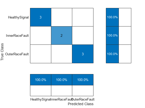
Use the test features to identify the faulty signals and analyze the accuracy of the classifier.
predictedLabels = predict(SVMModel,testMatrixNorm);

figure
cm = confusionchart(testResponse,predictedLabels, ...
ColumnSummary="column-normalized",RowSummary="row-normalized");

Calculate the classifier accuracy.
accuracy = trace(cm.NormalizedValues)/sum(cm.NormalizedValues,"all");
fprintf("The classification accuracy on the test partition is %2.1f%%",accuracy*100)
The classification accuracy on the test partition is 100.0%
Train LSTM Network Using Multidomain Features
Set Up Feature Extraction Objects for Training LSTM Network
Each signal in the signalDatastore object sds has around 150,000 samples. Window each signal into 2000-sample signal frames and extract multidomain features from it using all three feature extractors. You can achieve this by setting the FrameSize for all three feature extractors to 2000.
timeFE.FrameSize = 2000;
freqFE.FrameSize = 2000;
timeFreqFE.FrameSize = 2000;
Features extracted from frames correspond to a sequence of features over time that have lower dimension than the original signal. The dimension reduction helps the LSTM network to train faster. The workflow follows these steps:
Split the signal datastore and labels into training and test sets.
For each signal in the training and test sets, use all three feature extractor objects to extract features for multiple signal frames. Concatenate the multidomain features to obtain the feature matrix.
Normalize the training and testing feature matrices.
Train the recurrent deep learning network using the labels and feature matrices.
Classify the signals using the trained network.
Split the labels into training and testing sets. Use 70% of the labels for training set and the remaining 30% for testing data. Use splitlabels to obtain the desired partition of the labels. This guarantees that each split data set contains similar label proportions as the entire data set. Obtain the corresponding datastore subsets from the signalDatastore object. Reset the random number generator for reproducible results.
rng("default")

splitIndices = splitlabels(labels,0.7,"randomized");
trainIdx = splitIndices{1};
countlabels(labels(splitIndices{1}))
ans=3×3 table
      Healthy     8    33.3333
    InnerRace     5    20.8333
    OuterRace    11    45.8333
testIdx = splitIndices{2};
countlabels(labels(splitIndices{2}))ans=3×3 table
Healthy 4 40
InnerRace 2 20
OuterRace 4 40
trainDs = subset(sds,trainIdx);
trainLabels = labels(trainIdx);
testDs = subset(sds,testIdx);
testLabels = labels(testIdx);
Use the feature extractor objects to split each input signal in the training signalDatastore object into frames, and obtain a multidomain feature matrix. The feature vector extracted from each frame represents the signal segment and has significantly less number of samples. Therefore, using frame features to train the LSTM network is faster and computationally efficient (less number of hidden units) and helps performing a successful classification.
Extract Multidomain Features
Obtain features from the training datastore using all three feature extractors.
trainFeatures = cellfun(@(a,b,c) [a b c], extract(timeFE,trainDs), ...
    extract(freqFE,trainDs),extract(timeFreqFE,trainDs),UniformOutput=false);
Follow the same workflow to obtain test features.
testFeatures = cellfun(@(a,b,c) [a b c], extract(timeFE,testDs), ...
    extract(freqFE,testDs),extract(timeFreqFE,testDs),UniformOutput=false);
Normalize the training and testing features using the mean and standard deviation of the training features.
% Compute normalization parameters from training data
trainMatrix = cell2mat(trainFeatures);
featureMean = mean(trainMatrix,1,"omitnan");
featureStd = std(trainMatrix,0,1,"omitnan");

% Handle zero-variance features
zeroVarIdx = featureStd == 0;
featureStd(zeroVarIdx) = 1;  % Avoid division by zero

% Normalize training sequences
trainFeaturesNorm = cell(size(trainFeatures));
for i = 1:numel(trainFeatures)
    trainFeaturesNorm{i} = (trainFeatures{i} - featureMean)./ featureStd;
    trainFeaturesNorm{i}(~isfinite(trainFeaturesNorm{i})) = 0;
end

% Normalize test sequences using training parameters
testFeaturesNorm = cell(size(testFeatures));
for i = 1:numel(testFeatures)
    testFeaturesNorm{i} = (testFeatures{i} - featureMean)./ featureStd;
    testFeaturesNorm{i}(~isfinite(testFeaturesNorm{i})) = 0;
end
Train LSTM Network
Train the network using the training features and their corresponding labels.
numFeatures = size(trainFeatures{1},2);
numClasses = 3;
layers = [ ...
sequenceInputLayer(numFeatures)
lstmLayer(50,OutputMode="last")
fullyConnectedLayer(numClasses)
softmaxLayer];
options = trainingOptions("adam", ...
Shuffle="every-epoch", ...
Plots="training-progress", ...
ExecutionEnvironment="cpu", ...
MaxEpochs=100, ...
Verbose=false);
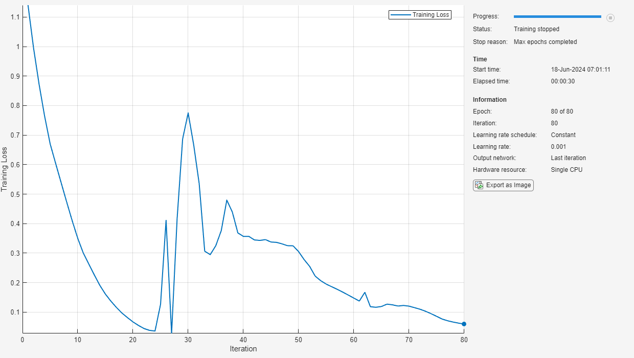
net = trainnet(trainFeaturesNorm,trainLabels,layers,"crossentropy",options);
Use the trained network to classify the signals in the testing data set and analyze the accuracy of the network.
scores = minibatchpredict(net,testFeaturesNorm);
classNames = categories(labels);
predTest = scores2label(scores,classNames);

figure
cm = confusionchart(testLabels,predTest, ...
ColumnSummary="column-normalized",RowSummary="row-normalized");
Calculate the classifier accuracy.
accuracy = trace(cm.NormalizedValues)/sum(cm.NormalizedValues,"all");
fprintf("The classification accuracy on the test partition is %2.1f%%",accuracy*100)
The classification accuracy on the test partition is 100.0%
References
[1] Cheng, Cheng, Guijun Ma, Yong Zhang, Mingyang Sun, Fei Teng, Han Ding, and Ye Yuan. “A Deep Learning-Based Remaining Useful Life Prediction Approach for Bearings.” IEEE/ASME Transactions on Mechatronics 25, no. 3 (June 2020): 1243–54. https://doi.org/10.1109/TMECH.2020.2971503
[2] Riaz, Saleem, Hassan Elahi, Kashif Javaid, and Tufail Shahzad. "Vibration Feature Extraction and Analysis for Fault Diagnosis of Rotating Machinery - A Literature Survey." Asia Pacific Journal of Multidisciplinary Research 5, no. 1 (2017): 103–110.
[3] Caesarendra, Wahyu, and Tegoeh Tjahjowidodo. “A Review of Feature Extraction Methods in Vibration-Based Condition Monitoring and Its Application for Degradation Trend Estimation of Low-Speed Slew Bearing.” Machines 5, no. 4 (December 2017): 21. https://doi.org/10.3390/machines5040021
See Also
Functions
confusionchart|pspectrum(Signal Processing Toolbox) |signalDatastore(Signal Processing Toolbox) |trainingOptions|trainnet|transform(Signal Processing Toolbox)
Objects
signalTimeFeatureExtractor(Signal Processing Toolbox) |signalFrequencyFeatureExtractor(Signal Processing Toolbox) |signalTimeFrequencyFeatureExtractor(Signal Processing Toolbox)
Topics
- Vibration Analysis of Rotating Machinery (Signal Processing Toolbox)
- Time-Frequency Feature Embedding with Deep Metric Learning