Accelerate Signal Feature Extraction and Classification Using a Parallel Pool of Workers

Introduction

This example extends the Machine Learning and Deep Learning Classification Using Signal Feature Extraction Objects example by showing how to compute features and train models using a parallel pool of CPU workers. Visit that example to read the details of the problem and the dataset.

Download and Prepare the Data

The data set contains acceleration signals collected from rotating machines in bearing test rig and real-world machines such as oil pump bearing, intermediate speed bearing, and a planet bearing. There are 34 files in total. The signals in the files are sampled at fs = 25 Hz. The filenames describe the signals they contain:

Download the data files into your temporary directory, whose location is specified by the tempdir command in MATLAB®. If you want to place the data files in a folder different from tempdir, change the directory name in the subsequent instructions. Create a signalDatastore object to access the data in the files and obtain the labels.

dataURL = "https://www.mathworks.com/supportfiles/SPT/data/rollingBearingDataset.zip";
datasetFolder = fullfile(tempdir,'rollingBearingDataset');
zipFile = fullfile(tempdir,'rollingBearingDataset.zip');
if ~exist(datasetFolder,'dir')
    websave(zipFile,dataURL);
    unzip(zipFile,datasetFolder);
end

Create a signalDatastore object to access the data in the files and obtain the labels.

sds = signalDatastore(datasetFolder);

The dataset filenames contain the label name. Get a list of labels from the filenames in the datastore using the filenames2labels function. Shorten the labels for better display using the function getShortenedLabels.

labels = filenames2labels(sds,ExtractBefore='_'); 
labels = getShortenedLabels(labels);

Setup for Feature Extraction Objects

In this section you set up the feature extractors that extract multidomain features from the signals. Use these features to implement machine learning and deep learning solutions that classify signals as healthy, as having inner race faults, or as having outer race faults [3].

Use the signalTimeFeatureExtractor, signalFrequencyFeatureExtractor, and signalTimeFrequencyFeatureExtractor objects to extract features from all the signals.

Create a signalTimeFeatureExtractor to extract time-domain features.

timeFE = signalTimeFeatureExtractor(SampleRate=25, ...
    RMS=true, ...
    ImpulseFactor=true, ...
    StandardDeviation=true, ...
    ClearanceFactor=true);

Create a signalFrequencyFeatureExtractor to extract frequency-domain features.

 freqFE = signalFrequencyFeatureExtractor(SampleRate=25, ...
    MedianFrequency=true, ...
    BandPower=true, ...
    PowerBandwidth=true, ...
    PeakAmplitude=true);

Create a signalTimeFrequencyFeatureExtractor to extract time-frequency domain features. To extract the time-frequency features, use a spectrogram with 90% leakage.

 timeFreqFE = signalTimeFrequencyFeatureExtractor(SampleRate=25, ...
    SpectralKurtosis=true, ...
    SpectralSkewness=true, ...
    SpectralFlatness=true, ...
    TFRidges=true, ...
    ScaleSpectrum=true);

setExtractorParameters(timeFreqFE,"spectrogram",Leakage=0.9);

Train an SVM Classifier Using Multidomain Features

Extract Multidomain Features

In this subsection, you extract multidomain features using a single CPU worker and a parallel pool of CPU workers and measure the computation times.

Extract features using a single CPU worker.

tStart = tic;
cellfun(@(a,b,c) [a b c],extract(timeFE,sds),extract(freqFE,sds),...
    extract(timeFreqFE,sds),UniformOutput=false);
tCPU = toc(tStart);

Repeat the process using a parallel pool of CPU workers. Set the UseParallel flag in the extract functions of all the feature extractors to true. Start a parallel pool of workers before you start measuring the computation time because the parallel pool can take some time to start.

if isempty(gcp("nocreate"))
    parpool("Processes");
end

Starting parallel pool (parpool) using the 'Processes' profile ...
28-Jun-2024 09:49:21: Job Queued. Waiting for parallel pool job with ID 1 to start ...
28-Jun-2024 09:50:22: Job Queued. Waiting for parallel pool job with ID 1 to start ...
28-Jun-2024 09:51:23: Job Queued. Waiting for parallel pool job with ID 1 to start ...
28-Jun-2024 09:52:24: Job Queued. Waiting for parallel pool job with ID 1 to start ...
28-Jun-2024 09:53:24: Job Queued. Waiting for parallel pool job with ID 1 to start ...
28-Jun-2024 09:54:25: Job Queued. Waiting for parallel pool job with ID 1 to start ...
28-Jun-2024 09:55:26: Job Queued. Waiting for parallel pool job with ID 1 to start ...
Connected to parallel pool with 6 workers.

Obtain multidomain features using a parallel pool of workers

tStart = tic;
SVMFeatures = cellfun(@(a,b,c) [a b c], extract(timeFE,sds,UseParallel=true), ...
    extract(freqFE,sds,UseParallel=true),extract(timeFreqFE,sds,UseParallel=true), ...
    UniformOutput=false);
tPool = toc(tStart);

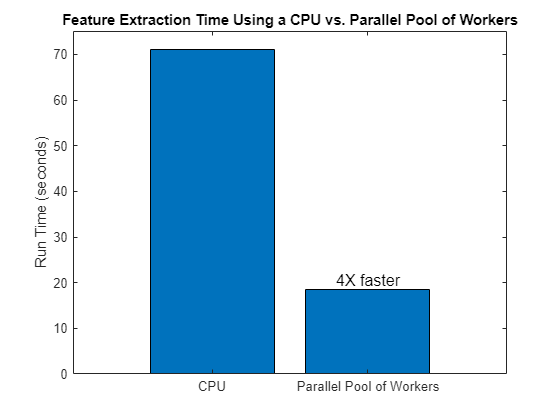
Compare the run times to see the speedup obtained when a parallel pool of CPU workers is used for feature extraction.

bar(["CPU" "Parallel Pool of Workers"],[tCPU tPool],0.8,FontSize=12,...
    Labels = ["" (num2str(round(tCPU/tPool))+"X faster")])
title("Feature Extraction Time Using a CPU vs. Parallel Pool of Workers")
ylabel("Run Time (seconds)")

Train an SVM Classifier Model

In this subsection, you obtain multidomain feature tables that are used to train a multiclass SVM classifier and observe the classification accuracy.

Obtain the feature table from the multidomain feature matrix.

featureMatrix = cell2mat(SVMFeatures);
featureTable = array2table(featureMatrix);

Split the feature table into training and testing feature data sets. Obtain their corresponding labels. Reset the random number generator for reproducible results.

rng default
cvp = cvpartition(labels,Holdout=0.25);

trainingPredictors = featureTable(cvp.training,:);
trainingResponse = labels(cvp.training,:);

testResponse = labels(cvp.test,:);
testPredictors = featureTable(cvp.test,:);

Use the training features to train an SVM classifier using a single CPU worker.

SVMModel = fitcecoc(trainingPredictors,trainingResponse);

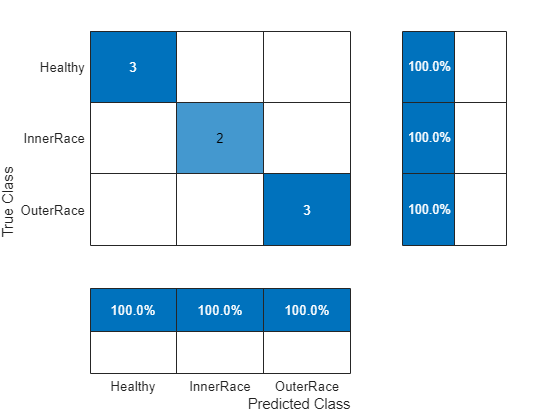
Use the test features to analyze the accuracy of the SVM classifier.

predictedLabels = predict(SVMModel,testPredictors);

figure
confusionchart(testResponse,predictedLabels, ...
    ColumnSummary="column-normalized",RowSummary="row-normalized");

Train an LSTM Network Using Features

Set Up Feature Extraction Objects for Training an LSTM Network

Each signal in the signalDatastore object sds has around 150,000 samples. Window each signal into 1000-sample frames and extract multidomain features from it. Set FrameSize for all three feature extractors to 1000 to achieve the signal framing.

timeFE.FrameSize = 1000;
freqFE.FrameSize = 1000;
timeFreqFE.FrameSize = 1000;

Features extracted from frames correspond to a sequence of features over time that has lower dimension than the original signal. The dimension reduction helps the LSTM network to train faster. The workflow in this section follows these steps:

Split the labels into training and testing sets. Use 70% of the labels for training set and the remaining 30% for testing data. Use splitlabels to obtain the desired partition of the labels. This guarantees that each split data set contains similar label proportions as the entire data set. Obtain the corresponding datastore subsets from the signalDatastore object. Reset the random number generator for reproducible results.

rng default

splitIndices = splitlabels(labels,0.7,"randomized");

trainIdx = splitIndices{1};
trainLabels = labels(trainIdx);
testIdx = splitIndices{2};
testLabels = labels(testIdx);

Obtain the training and testing signalDatastore subsets from sds for multidomain feature extraction from the signals in them.

trainDs = subset(sds,trainIdx); 
testDs = subset(sds,testIdx);

Extract Multidomain Features

Obtain multidomain training and testing features from the signalDatastore subsets using a parallel pool of workers.

trainFeatures = cellfun(@(a,b,c) [a b c], extract(timeFE,trainDs,UseParallel=true),...
    extract(freqFE,trainDs,UseParallel=true),extract(timeFreqFE,trainDs,UseParallel=true),...
    UniformOutput=false);

testFeatures = cellfun(@(a,b,c) [a b c], extract(timeFE,testDs,UseParallel=true),...
    extract(freqFE,testDs,UseParallel=true),extract(timeFreqFE,testDs,UseParallel=true),...
    UniformOutput=false);

Train an LSTM network

Train an LSTM network using the training features and their corresponding labels.

numFeatures = size(trainFeatures{1},2);
numClasses = 3;
 
layers = [ ...
    sequenceInputLayer(numFeatures)
    lstmLayer(50,OutputMode="last")
    fullyConnectedLayer(numClasses)
    softmaxLayer];
 
options = trainingOptions("adam", ...
    Shuffle="every-epoch", ...    
    Plots="training-progress", ...
    ExecutionEnvironment="cpu", ...
    MaxEpochs=80, ...
    Verbose=false);

net = trainnet(trainFeatures,trainLabels,layers,"crossentropy",options);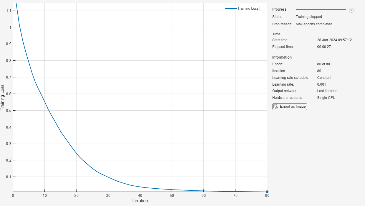

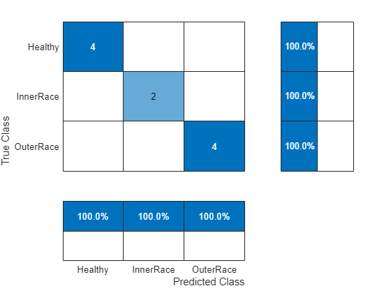
Use the trained network to classify the signals in the test dataset and analyze the accuracy of the network.

scores = minibatchpredict(net,testFeatures);
classNames = categories(labels);
predTest = scores2label(scores,classNames);
 
figure
cm = confusionchart(testLabels,predTest,...
    ColumnSummary="column-normalized",RowSummary="row-normalized");

Summary

This example shows how the feature extraction process can be accelerated using a parallel pool of CPU workers. To observe the performance acceleration for feature extraction and model training when a GPU is used, visit the Accelerate Signal Feature Extraction and Classification Using a GPU example.

References

[1] Cheng, Cheng, Guijun Ma, Yong Zhang, Mingyang Sun, Fei Teng, Han Ding, and Ye Yuan. “A Deep Learning-Based Remaining Useful Life Prediction Approach for Bearings.” IEEE/ASME Transactions on Mechatronics 25, no. 3 (June 2020): 1243–54. https://doi.org/10.1109/TMECH.2020.2971503

[2] Riaz, Saleem, Hassan Elahi, Kashif Javaid, and Tufail Shahzad. "Vibration Feature Extraction and Analysis for Fault Diagnosis of Rotating Machinery - A Literature Survey." Asia Pacific Journal of Multidisciplinary Research 5, no. 1 (2017): 103–110.

[3] Caesarendra, Wahyu, and Tegoeh Tjahjowidodo. “A Review of Feature Extraction Methods in Vibration-Based Condition Monitoring and Its Application for Degradation Trend Estimation of Low-Speed Slew Bearing.” Machines 5, no. 4 (December 2017): 21. https://doi.org/10.3390/machines5040021

[4] Tian, Jing, Carlos Morillo, Michael H. Azarian, and Michael Pecht. “Motor Bearing Fault Detection Using Spectral Kurtosis-Based Feature Extraction Coupled With K-Nearest Neighbor Distance Analysis.” IEEE Transactions on Industrial Electronics 63, no. 3 (March 2016): 1793–1803. https://doi.org/10.1109/TIE.2015.2509913

[5] Li, Yifan, Xin Zhang, Zaigang Chen, Yaocheng Yang, Changqing Geng, and Ming J. Zuo. “Time-Frequency Ridge Estimation: An Effective Tool for Gear and Bearing Fault Diagnosis at Time-Varying Speeds.” Mechanical Systems and Signal Processing 189 (April 2023): 110108. https://doi.org/10.1016/j.ymssp.2023.110108

Helper Function

getShortenedLabels – This function shortens the labels for better display on confusion charts.

function shortenedLabels = getShortenedLabels(labels)
%   This function is only intended support examples in the Signal
%   Processing Toolbox. It may be changed or removed in a future release

shortenedLabels = string(size(labels));
labels = string(labels);

for idx=1:numel(labels)
    if labels(idx) == "HealthySignal"
        str2erase = "Signal";
    else
        str2erase = "Fault";
    end
    shortenedLabels(idx) = erase(labels(idx),str2erase);
end

shortenedLabels = categorical(shortenedLabels);
shortenedLabels = shortenedLabels(:);
end