Uncertainty Quantification for ECG Signal Classification
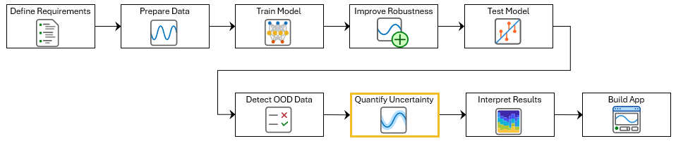
This example shows how to use split conformal prediction (SCP) with a pretrained ECG signal classifier to quantify uncertainty in the predictions of the network. This example is step seven in a series of examples that take you through an ECG signal classification workflow. This workflow classifies ECG signals as either Normal ("N") or Atrial Fibrillation ("A"). This example follows the Out-of-Distribution Detection for ECG Signal Classification example. For more information about the full workflow, see ECG Signal Classification Using Deep Learning.
To open this example, open ECG Signal Classification Using Deep Learning and navigate to scripts\S7_ConformalPrediction. Alternatively, if you already have MATLAB open, then run
openExample("deeplearning_shared/ECGSignalClassificationUsingDeepLearningExample")This project contains all of the steps for this workflow. You can run the scripts in order or each one independently.
Deep learning classifiers typically return a single class label for each input. In ECG signal classification, this means assigning one label to each time series. However, these predictions do not indicate how confident the model is. Misclassifications can occur due to noise, overlapping clinical features, or model limitations. Labeling an abnormal rhythm as normal can have serious clinical consequences. To reduce the risk of incorrect predictions, predictions should also indicate how uncertain the model is, so that you can identify cases where the model may be unsure.
One way to express uncertainty is to return a prediction set instead of a single label. A prediction set contains all labels that are plausible for a given input, based on the model and a user-specified error rate. The error rate is the maximum proportion of future predictions that exclude the true label. For example, an error rate of 0.1 means that, on average, at most 10% of prediction sets will not contain the true label.
Split conformal prediction (SCP) is a distribution-free, model-agnostic method that constructs prediction sets with statistical guarantees on this error rate. This example uses the SCP technique adaptive prediction sets (APS). APS uses the softmax probabilities of the model to build prediction sets that adapt to the confidence of the model. This results in small sets when the model is confident and large sets when it is uncertain. For more information, see [1].
This example shows how to apply SCP to a pretrained ECG classifier by following these steps:
Compute nonconformity scores — For each calibration example, calculate the APS score by summing the predicted probabilities of all classes with equal or higher softmax probability than the true label. A higher APS score means that the true label was not among the top predictions, indicating low model confidence.
Compute conformal quantile — Determine the score threshold (quantile) from the calibration scores that guarantees that the error rate does not exceed the target level.
Construct prediction sets — For each new input, sort class probabilities in descending order and include classes until the cumulative sum exceeds the threshold. This produces sets that adapt to model confidence.
Verify empirical coverage — Evaluate the prediction sets of the test data to confirm that the observed error rate is at or below the specified level.
SCP provides statistical validity guarantees only when the test data comes from the same distribution as the calibration data. For this reason, you should only apply SCP to in-distribution data. To determine if your data is in-distribution, see Out-of-Distribution Detection for ECG Signal Classification.
Load the calibration and test data. If you have run the previous step, then the example uses the data that you prepared earlier. Otherwise, the example prepares the data as shown in Prepare Data for ECG Signal Classification.
if  ~exist("XCalib","var") || ~exist("TCalib","var") || ~exist("XTest","var") || ~exist("TTest","var")
    [~,~,XCalib,TCalib,XTest,TTest] = prepareECGData;
end
Load a pretrained network. If you have run the previous training step, Improve Adversarial Robustness of Deep Learning Network for ECG Signal Classification, then the example uses your trained network. Otherwise, load a pretrained network. The network has been trained using the steps shown in Improve Adversarial Robustness of Deep Learning Network for ECG Signal Classification.
if ~exist("netRobust","var")
    load("adversariallyTrainedECGNetwork.mat");
end
Compute Nonconformity Scores
Use the calibration set of ECG signals to compute conformity scores by using the custom nonconformityScores function, which is defined at the end of this example. The function accepts a deep neural network (netRobust), ECG signals (XCalib), and true class labels for the calibration set (TCalib). For each observation, the function computes the APS nonconformity score, which is the minimum cumulative probability mass that must include the true class when classes are sorted by predicted probability. Larger scores indicate higher nonconformity because a larger probability mass is required to cover the true label.
scores = nonconformityScores(netRobust,XCalib,TCalib);
Compute Conformal Quantile
Use the nonconformity scores and error rate to compute the conformal threshold using the custom conformalQuantile function, which is defined at the end of this example. The function accepts a vector of nonconformity scores (scores) and a desired error rate (errorRate). The function returns the conformal threshold.
The threshold defines the minimum cumulative probability mass that each prediction set must include to ensure that, on average, the set excludes the true label no more than the specified error rate. Therefore, if you include classes until their cumulative probability exceeds this threshold, then your prediction sets will satisfy the error rate guarantee. A lower target error rate requires a higher threshold, resulting in larger prediction sets.
errorRate = 0.75;
threshold = conformalQuantile(scores,errorRate)
0.75;
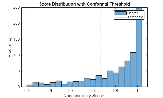
threshold = conformalQuantile(scores,errorRate)threshold = single
0.8314
Plot the distribution of calibration scores and mark the threshold.
figure
histogram(scores, 20)
xline(threshold,"--")
xlabel("Nonconformity Scores")
ylabel("Frequency")
title("Score Distribution with Conformal Threshold")
legend("Scores","Threshold")
Construct Prediction Sets for the Test Set
Apply the conformal threshold to the test set by using the custom conformalPredict function, which is defined at the end of this example. This function accepts a deep neural network (netRobust), a set of ECG signals (XTest), a conformal threshold (threshold), and a vector of class names (classNames).
The function returns three cell arrays. The first array contains the prediction set for each test sample as a categorical vector. The second array contains the softmax probabilities for the labels in each prediction set in the same order. The third array contains all the class scores, in the order specified by the class names.
classNames = categories(TTest);
[YTestSet,YTestScores,allScores] = conformalPredict(netRobust,XTest,threshold,classNames);
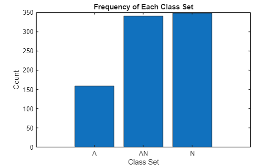
For each ECG signal, the prediction set will contain either N, A, or both. If the set contains only one class, then for the specified error rate, the classifier is confident in that label. If the set contains both classes, then the model is unable to confidently distinguish between "N" and "A" for that signal. For example, if the top prediction of a classifier is N, but the prediction set is [A,N], then the model cannot confidently rule out atrial fibrillation. This is especially important in clinical settings, where missing an atrial fibrillation episode (a false negative) can have serious consequences.
Plot the number of signals that have the label set "A", "N", or "A and N" (represented by "AN" in the plot).
combineClasses = strings(size(YTestSet));
for i = 1:numel(YTestSet)
    x = YTestSet{i};
    sortedChars = sort(char(x));
    combineClasses(i) = string(sortedChars');
end

[uniqueElements,~,idx] = unique(combineClasses);
counts = accumarray(idx(:),1);

figure
bar(counts)
xticks(1:numel(uniqueElements))
xticklabels(uniqueElements)

xlabel("Class Set")
ylabel("Count")
title("Frequency of Each Class Set")
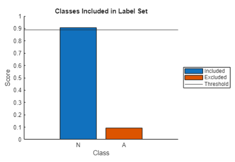
To better understand the prediction set, visualize the cumulative probability mass for an individual test signal by using the explainPredictionSet function, which is defined at the end of this example. This function takes as input the class scores, the class names, and the threshold.
The function returns a plot showing the score for each class and a horizontal line showing the threshold. Conformal prediction adds the classes in order of descending probability, and all classes up to and including the first one that causes the cumulative probability to meet or exceed the threshold are included in the prediction set. In the plot, blue bars represent included classes, and red bars represent excluded classes. If both the bars are blue, then the label set for that signal contains both classes.
Explain the prediction set of idx observation.
idx = 711;
explainPredictionSet(allScores{idx},categories(TTest),threshold);
711;
explainPredictionSet(allScores{idx},categories(TTest),threshold);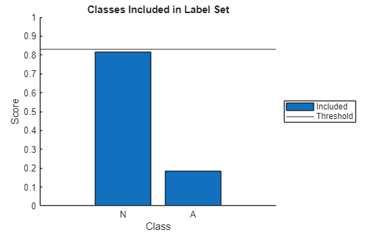
Verify Empirical Coverage
For the test set, check how often the true class label is not included in the prediction set. The proportion of such cases is the empirical error rate.
numTest = numel(TTest);
containsTrueLabel = false(numTest,1);

for i = 1:numTest
    containsTrueLabel(i) = any(YTestSet{i} == TTest(i));
end

empiricalErrorRate = 1- mean(containsTrueLabel);
disp("Target error rate: " + errorRate)
Target error rate: 0.75
disp("Empirical error rate: " + empiricalErrorRate)Empirical error rate: 0.081368
If the empirical error rate is less than or equal to the target error rate, then that confirms that the conformal prediction method provides valid uncertainty quantification for your ECG classifier.
In the next step of the workflow, you will use the gradient-weighted class activation mapping (Grad-CAM) technique to explain the most likely prediction.
Supporting Functions
Compute Nonconformity Scores
The nonconformityScores function accepts a deep neural network (net), ECG signals (XCalib) and true class labels for the calibration set (TCalib). For each observation, the function computes the APS nonconformity score, which is the minimum cumulative probability mass needed to include the true class when classes are sorted by predicted probability. Larger scores indicate higher nonconformity because the true label requires more probability mass to be covered.
The nonconformityScores function performs these steps:
Predict class probabilities for each calibration sample.
Sort the predicted probabilities in descending order.
For each sample, determine the rank of the true class in the sorted list.
Compute the cumulative sum of the sorted probabilities.
For each sample, extract the cumulative probability up to and including the true class. This value is the APS nonconformity score for that sample.
function scores = nonconformityScores(net,XCalib,TCalib)
YCalib = minibatchpredict(net,XCalib,InputDataFormats="CTB");
[sortedPredictions,sortedIndex] = sort(YCalib,2,"descend");
[~,trueClassRank] = max(sortedIndex == double(TCalib),[],2);
sortedSum = cumsum(sortedPredictions,2);
trueClassIndex = sub2ind(size(sortedSum),(1:length(sortedIndex))',trueClassRank);
scores = sortedSum(trueClassIndex);
end
Compute Conformal Quality
The conformalQuantile function accepts a vector of nonconformity scores (calibrationScores) and a desired error rate (errorRate). This function returns the conformal threshold. The threshold defines the minimum cumulative probability mass that each prediction set must include to ensure that, on average, the set excludes the true label at a rate no higher than the specified error rate. Therefore, if you include classes until their cumulative probability exceeds this threshold, your prediction sets will satisfy the error rate guarantee. A lower target error rate requires a higher threshold, resulting larger prediction sets.
The conformalQuantile function performs these steps:
Sort the nonconformity scores in ascending order.
Find the index corresponding to the desired error rate.
Select the score at this index as the conformal threshold.
function threshold = conformalQuantile(calibrationScores,errorRate)
sortedScores = sort(calibrationScores,"ascend");
numObservations = numel(calibrationScores);
coverageIndex = ceil((numObservations+1)*(1-errorRate));
threshold = sortedScores(coverageIndex);
end
Apply Conformal Prediction Threshold
The conformalPredict function accepts a deep neural network (net), a set of ECG signals (X), a conformal threshold (threshold), and a vector of class names (classNames). The function returns three cell arrays. The first array contains the prediction set for each test sample as a categorical vector. The second array contains the softmax probabilities for the labels in each prediction set in the same order. The third array contains all the class scores, in the order specified by the class names.
This function performs these steps:
Predict class probabilities for each test sample.
Sort the predicted probabilities in descending order.
Compute the cumulative sum of the sorted probabilities for each sample.
For each sample, find the smallest set of top classes whose cumulative probability meets or exceeds the specified threshold.
For each sample, convert the selected class indices into class labels and return the labels and their probabilities.
function [predictionSets,predictionScores,allScores] = conformalPredict(net,X,threshold,classNames)
Y = minibatchpredict(net,X,InputDataFormats="CTB");

[sortedPredictions,sortedIndex] = sort(Y,2,"descend");
sortedSum = cumsum(sortedPredictions,2);

meetsThreshold = sortedSum >= threshold;
[~,cutoffIndex] = max(meetsThreshold,[],2);

numSamples = size(Y,1);
predictionSets = cell(1,numSamples);
predictionScores = cell(1,numSamples);
allScores = cell(1,numel(classNames));

for i = 1:numSamples
    includedIndex = sortedIndex(i,1:cutoffIndex(i));
    includedLabels = classNames(includedIndex);
    predictionSets{i} = categorical(includedLabels,classNames);
    predictionScores{i} = sortedPredictions(i, 1:cutoffIndex(i));
    allScores{i} = Y(i,:);
end
end
Explain Prediction Set
The explainPredictionSet function takes as input the class scores for a single signal (signalScores), class names (classes), and the threshold (threshold). The function returns a plot that shows the score for each class, with a horizontal line marking the threshold. Conformal prediction adds the classes in order of descending probability, and all classes up to and including the first one that causes the cumulative probability to meet or exceed the threshold are included in the prediction set. In the plot, blue bars represent included classes, and red bars represent excluded classes. If both the bars are blue, then the label set for that signal contains both classes.
The function performs these steps:
Sort the probability scores into descending order.
Find the classes to include in order to meet the threshold.
Plot the scores in a bar plot. Blue bars represent included classes, and red bars represent excluded classes.
function explainPredictionSet(signalScores,classes,threshold)

% Sort probabilities
[sortedProbs,sortedIdx] = sort(signalScores,"descend");
sortedNames = classes(sortedIdx);
cumProb = cumsum(sortedProbs);

% Find smallest top-k set meeting threshold
cutoff = find(cumProb >= threshold,1,"first");

if isempty(cutoff)
    cutoff = numel(sortedProbs);
end

% Plot results
RGB = orderedcolors("gem");
colorBar = repmat(RGB(2,:),numel(cumProb),1);
colorBar(1:cutoff,:) = repmat(RGB(1,:),cutoff,1);

figure
labels = ["Included","Excluded"];

hold on
if cutoff ~= numel(classes)
    for i = 1:numel(sortedIdx)
        bb(i) = bar(i,sortedProbs(i),FaceColor=colorBar(i,:));
    end
    legend(bb,labels{cutoff:end},Location="eastoutside");
else
    bb = bar(1:cutoff,sortedProbs,FaceColor=colorBar(1,:));
    legend(bb,labels{1},Location="eastoutside");
end

yline(threshold,"-",DisplayName="Threshold");
xticks(1:numel(sortedNames))
xticklabels(sortedNames)
ylabel("Score")
xlabel("Class")
ylim([0,1])
title("Classes Included in Label Set")
hold off
end
References
[1] Romano, Yaniv, et al. “Classification with Valid and Adaptive Coverage.” arXiv:2006.02544, arXiv, 3 Jun. 2020. arXiv.org, https://doi.org/10.48550/arXiv.2006.02544.
See Also
testnet | networkDistributionDiscriminator | isInNetworkDistribution