Quantify Uncertainty in Object Detection Using Split Conformal Prediction
This example shows how to apply split conformal prediction (SCP) to an object detection model to quantify uncertainty in the predicted labels and bounding boxes.
Deep learning models typically produce a single prediction for each input. For example, in object detection tasks, the model outputs a single label and a bounding box. However, this top prediction can be wrong due to factors such as data noise, object ambiguity, and model limitations. Quantifying prediction uncertainty helps with assessing prediction reliability and supports more robust decision making.
SCP is a distribution-free, model-agnostic method for building prediction sets (or intervals for continuous responses). Given an acceptable error rate, , and a calibration set of size , SCP computes nonconformity scores for the calibration data and uses their -th quantile to define a threshold that determines the size of the prediction set. Over repeated trials, the resulting prediction sets contain the true value with a probability of at least . This coverage guarantee holds as long as the calibration data is exchangeable with the test data. For more information on SCP, see Uncertainty Estimation for Regression (Statistics and Machine Learning Toolbox).
You can use SCP with any predictive model, including neural networks, decision trees, and support vector machines. In this example, you apply SCP to an object detection model. For each detection, SCP returns:
A set of candidate labels that is expected to include the true label, even if the top prediction of the model is incorrect.
Two nested bounding boxes that define an interval expected to contain the true bounding box.
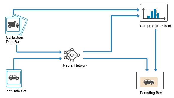
In this example, you:
Prepare data — Split the dataset into training, calibration, and test sets.
Train detector — Train an object detector on the training set.
Calibrate detector — Use the calibration set to calibrate the model by computing nonconformity scores and estimating a quantile threshold for the desired error rate.
Evaluate detector — Evaluate the model on the test set by constructing prediction sets for class labels and intervals for bounding boxes and then checking how often these contain the true value.
Prepare Data
This example uses synthetic data that was generated using a FlightGear simulation and a Simulink model. The images simulate the view from a forward-facing camera mounted on an aircraft during taxiing and ground operations. Each image contains one or more airport signs. For more information about the Simulink model used to generate these images, see Runway Sign Classifier: Certify an Airborne Deep Learning System (DO Qualification Kit).
The aim is to train a model than can detect the signs and classify them into one of two categories:
Mandatory signs — Indicate instructions that must be followed, such as stop or hold positions.
Informational signs — Provide guidance or situational information, such as taxiway identifiers or direction indicators.
Download and extract the generated data.
zipFile = matlab.internal.examples.downloadSupportFile("nnet","data/visualsignrecognitiondataset.zip");

dataPath = fullfile(tempdir,"Data");
unzip(zipFile,dataPath);
addpath(genpath(dataPath));
Load the raw data labels.
rawDataLabels = load("dataLabels.mat");
head(rawDataLabels.dataTable)
imageFilename informational mandatory
__________________________________________________ _________________ _________________
"KBOS7_SPRN_DAWN_RAIN_DIST10_SIDE0.3_AGL1.jpg" {0×0 double } {[ 98 129 46 23]}
"KBOS7_SPRN_DAWN_RAIN_DIST11_SIDE0.68_AGL1.6.jpg" {0×0 double } {[ 92 141 42 21]}
"KBOS7_SPRN_DAWN_RAIN_DIST12_SIDE0.71_AGL1.3.jpg" {0×0 double } {[ 95 136 38 19]}
"KBOS7_SPRN_DAWN_RAIN_DIST13_SIDE0.11_AGL1.1.jpg" {0×0 double } {[112 130 36 17]}
"KBOS7_SPRN_DAWN_RAIN_DIST14_SIDE0.65_AGL1.7.jpg" {0×0 double } {[123 140 32 16]}
"KBOS7_SPRN_DAWN_RAIN_DIST15_SIDE0.34_AGL1.9.jpg" {0×0 double } {[118 143 30 15]}
"KBOS19_SPRN_DAWN_RAIN_DIST10_SIDE0.76_AGL2.jpg" {[118 150 53 21]} {0×0 double }
"KBOS19_SPRN_DAWN_RAIN_DIST11_SIDE0.08_AGL1.7.jpg" {[102 143 49 19]} {0×0 double }
dataTable contains three columns:
imageFilename— File paths to the JPG images.informational— Ground-truth bounding boxes for the informational signs, specified as an matrix. Each row is in the format , where is the top-left corner and is the width and height. If the image contains no informational signs, then the matrix is empty.mandatory— Ground-truth bounding boxes for mandatory signs, using the same format asinformational.
Set aside data for testing. Partition the data into a training set containing 60% of the data, a calibration set containing 20% of the data, and a test set containing the remaining 20% of the data. To partition the data, use the trainingPartitions function, which is attached to this example as a supporting file. To access this file, open the example as a live script.
numObservations = size(rawDataLabels.dataTable,1);
[idxTrain,idxCal,idxTest] = trainingPartitions(numObservations,[0.6 0.2 0.2]);

trainData = rawDataLabels.dataTable(idxTrain,:);
calibData = rawDataLabels.dataTable(idxCal,:);
testData = rawDataLabels.dataTable(idxTest,:);
Create a datastore for each of the training, calibration, and testing data. Use the imageDatastore function to manage image files and the boxLabelDatastore (Computer Vision Toolbox) function to provide the corresponding bounding boxes. To create the datastores, combine the image and the bounding boxes by using the combine function.
imdsTrain = imageDatastore(trainData{:,1});
bldsTrain = boxLabelDatastore(trainData(:,2:3));
dsTrain = combine(imdsTrain,bldsTrain);

imdsCalib = imageDatastore(calibData{:,1});
bldsCalib = boxLabelDatastore(calibData(:,2:3));
dsCalib = combine(imdsCalib,bldsCalib);

imdsTest = imageDatastore(testData{:,1});
bldsTest = boxLabelDatastore(testData(:,2:3));
dsTest = combine(imdsTest,bldsTest);
Use the transform function to resize the images and bounding boxes in each datastore. To preprocess the data, use the helper function preprocessData, which is provided at the end of this example.
inputSize = [128 128 3];

dsTrain = transform(dsTrain,@(data)preprocessData(data,inputSize));
dsCalib = transform(dsCalib,@(data)preprocessData(data,inputSize));
dsTest = transform(dsTest,@(data)preprocessData(data,inputSize));
Train Detector
Train a YOLO v2 object detector to recognize the informational and mandatory traffic signs in the training data.
Define YOLO v2 Network Architecture
Specify the network input size and output classes.
outputClasses = ["informational","mandatory"];
numClasses = numel(outputClasses);
Load a pretrained MobileNet-v2 network using the imagePretrainedNetwork function. This network acts as the base network and extracts feature maps from input images.
baseNetwork = imagePretrainedNetwork("mobilenetv2");Specify block_12_add as the feature layer. YOLO v2 attaches the detection subnetwork after this layer, replacing all subsequent layers in the base network. The block_12_add layer downsamples the feature maps by a factor of 16, balancing spatial resolution and feature strength for accurate object detection.
featureLayer = "block_12_add";Estimate anchor boxes from the training data by using the estimateAnchorBoxes (Computer Vision Toolbox) function. Anchor boxes define the initial shapes and sizes of the bounding boxes predicted by the detector.
anchorBoxes = estimateAnchorBoxes(dsTrain,3);
Create the YOLO v2 object detection network using yolov2ObjectDetector (Computer Vision Toolbox).
layers = yolov2ObjectDetector(baseNetwork,outputClasses,anchorBoxes,DetectionNetworkSource=featureLayer);
Specify Training Options
Specify the training options by using the trainingOptions object. To help you choose training options for your model, you can experiment with different configurations in the Experiment Manager app. For this example, use these options.
options = trainingOptions("adam", ...
    ExecutionEnvironment="auto", ...
    InitialLearnRate=0.001, ...
    MiniBatchSize=16, ...
    MaxEpochs=40, ...
    Shuffle="every-epoch", ...
    LearnRateDropFactor=0.1, ...
    LearnRateDropPeriod=10, ...
    LearnRateSchedule="piecewise", ...
    BatchNormalizationStatistics="moving", ...
    ResetInputNormalization=false, ...
    VerboseFrequency=30, ...
    Plots="training-progress");
Train Network
Train the object detector using the trainYOLOv2ObjectDetector (Computer Vision Toolbox) function.
detector = trainYOLOv2ObjectDetector(dsTrain,layers,options);
*************************************************************************
Training a YOLO v2 Object Detector for the following object classes:

* informational
* mandatory

Training on single CPU.
|========================================================================================|
|  Epoch  |  Iteration  |  Time Elapsed  |  Mini-batch  |  Mini-batch  |  Base Learning  |
|         |             |   (hh:mm:ss)   |     RMSE     |     Loss     |      Rate       |
|========================================================================================|
|       1 |           1 |       00:00:10 |         6.15 |         37.8 |          0.0010 |
|       3 |          30 |       00:01:39 |         1.80 |          3.2 |          0.0010 |
|       6 |          60 |       00:03:04 |         0.94 |          0.9 |          0.0010 |
|       9 |          90 |       00:04:31 |         0.69 |          0.5 |          0.0010 |
|      12 |         120 |       00:05:55 |         0.60 |          0.4 |          0.0001 |
|      15 |         150 |       00:07:19 |         0.57 |          0.3 |          0.0001 |
|      18 |         180 |       00:08:42 |         0.56 |          0.3 |          0.0001 |
|      21 |         210 |       00:10:05 |         0.54 |          0.3 |      1.0000e-05 |
|      24 |         240 |       00:11:29 |         0.53 |          0.3 |      1.0000e-05 |
|      27 |         270 |       00:12:53 |         0.53 |          0.3 |      1.0000e-05 |
|      30 |         300 |       00:14:14 |         0.52 |          0.3 |      1.0000e-05 |
|      33 |         330 |       00:15:36 |         0.53 |          0.3 |      1.0000e-06 |
|      36 |         360 |       00:17:01 |         0.52 |          0.3 |      1.0000e-06 |
|      39 |         390 |       00:18:25 |         0.52 |          0.3 |      1.0000e-06 |
|      40 |         400 |       00:18:54 |         0.52 |          0.3 |      1.0000e-06 |
|========================================================================================|
Training finished: Max epochs completed.
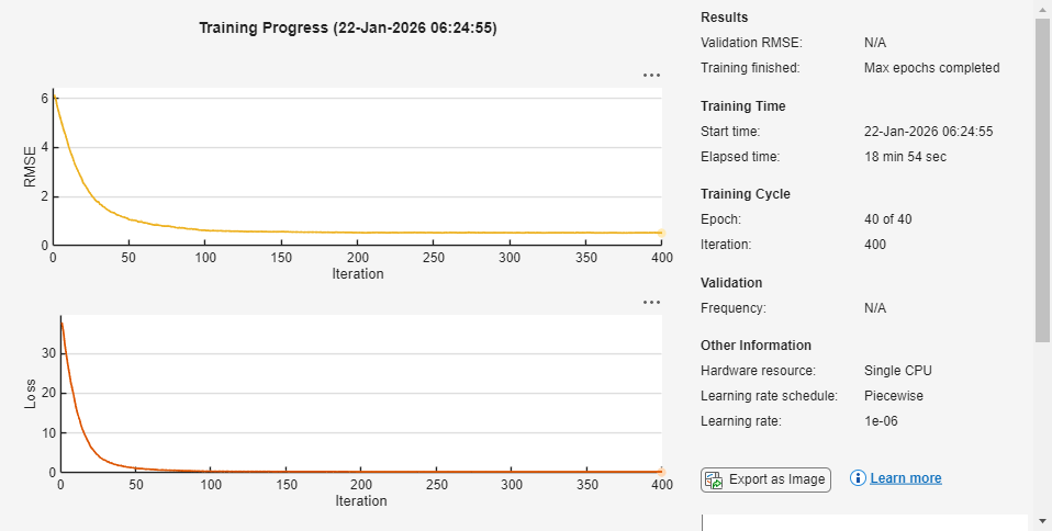
Detector training complete.
*************************************************************************
Calibrate Detector Using SCP
SCP uses a held-out calibration set to characterize how much the predictions of the model typically vary from the true values. For each calibration example, compute a nonconformity score that measures how dissimilar the prediction is from the ground truth. These scores form a reference distribution that reflect the uncertainty of the model. From this distribution, you can compute the quantile to obtain a threshold that corresponds to the acceptable error rate . Under the exchangeability assumption, this threshold allows you to construct prediction sets for new inputs that achieve the desired coverage.
Compute Nonconformity Scores
SCP provides valid coverage for any real-valued nonconformity score function, as long as you use the same score function during calibration and evaluation. However, the efficiency of the resulting prediction sets depends on the choice of score function. The SCP procedure is the same for all predictive models, but different score functions are better suited for different prediction tasks. In this example, you use the adaptive predictions set (APS) score [1] for class labels and the max-additive score for bounding boxes [2].
Use the helper function nonconformityScores, which is provided end of this example, to compute the label and bounding box nonconformity scores for the calibration set. The nonconformityScores function accepts a trained object detector (detector), a calibration datastore (dsCalib), a detection threshold (detectionThreshold), and an intersection-over-union (IoU) threshold (iouThreshold).
The function returns the nonconformity scores for the predicted class labels (labelScores) and bounding boxes (bboxScores) for each true positive detection in the calibration set.
labelScores— A column vector of size . The function computes each score from the predicted class probabilities of the model. If the model assigns a high probability to the true class, then the score is smaller. If the model assigns a high probability to the other classes, then the score is larger. Formally, the score is the cumulative probability of all classes ranked above the true class, plus the probability of the true class.bboxScores— A matrix of size . Each row contains the absolute difference between the predicted and true bounding box coordinates. A large score indicates a greater localization error.
Use the detectionThreshold parameter to exclude low-confidence predictions, so that only reliable detections contribute to the nonconformity scores. Set this value to the same value that you plan to use during inference when calling the detect (Computer Vision Toolbox) function, so the calibration statistics reflect your inference-time behavior.
Use the iouThreshold parameter to match only pairs with sufficient overlap, so that only meaningful matches contribute to the nonconformity scores. Set this value to the match the IoU threshold you want to use when you evaluate the detector with functions such as evaluateObjectDetection (Computer Vision Toolbox). This ensures that the calibration step uses the same matching criterion as your evaluation workflow.
detectionThreshold =0.25; iouThreshold =
0.5; [labelScores,bboxScores] = nonconformityScores(detector,dsCalib,detectionThreshold,iouThreshold);
Compute Conformal Quantile
Determine the conformal threshold, which translates the acceptable error rate into a rule for the constructing prediction set for the labels and the interval for the bounding boxes. Compute the threshold as the quantile of the nonconformity scores.
Use the helper function conformalQuantile, which is provided at the end of this example, to compute the conformal threshold for the label scores. This function takes as input a vector of nonconformity scores (calibrationScores) and a desired error rate (errorRate). The function returns the conformal threshold, which is the quantile corresponding to the desired error rate.
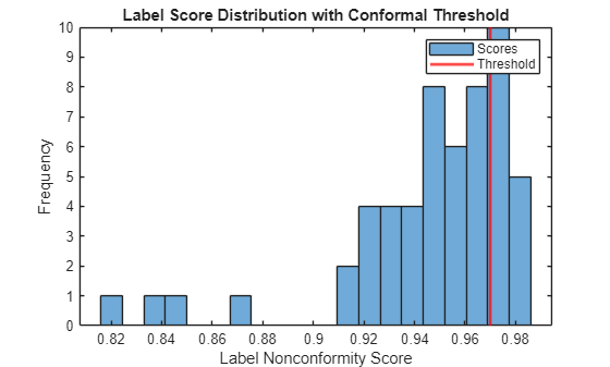
errorRate = 0.25;
labelThreshold = conformalQuantile(labelScores,errorRate)
0.25;
labelThreshold = conformalQuantile(labelScores,errorRate)labelThreshold = 0.9700
Plot the distribution of calibration scores and mark the threshold.
figure
histogram(labelScores,20)
xline(labelThreshold,"r",LineWidth=2)
xlabel("Label Nonconformity Score")
ylabel("Frequency")
title("Label Score Distribution with Conformal Threshold")
legend("Scores","Threshold")
Use the bounding box scores and significance level to compute the conformal threshold for the bounding boxes.
bboxThreshold = conformalQuantile(bboxScores,errorRate)
bboxThreshold =
3.5000
Evaluate Detector
Generate conformal prediction sets and intervals for the held-out test set, then assess the empirical miscoverage rates.
Construct Prediction Sets
To obtain conformal prediction sets and intervals, use the helper function conformalPredict, which is listed at the end of this example. This function accepts a trained object detector (detector), an input image (image), a detection threshold (detectionThreshold), a conformal threshold for the class labels (labelThreshold), and a conformal threshold for the bounding boxes (bboxThreshold). The function returns the conformal prediction set for the class labels and the conformal prediction interval for the bounding boxes for each detection.
Read an image from the test datastore and use the conformalPredict function to obtain conformal prediction sets and intervals.
image = read(dsTest);
gtbox = image{2};
image = image{1};

[labelSetsMask,labelSetsProb,bboxIntervals] = conformalPredict(detector,image,detectionThreshold,labelThreshold,bboxThreshold);
The labelSetMask output contains the conformal prediction sets for class labels. labelSetMask is an logical array, where labelSetMask(n,c) is true if class c is in the conformal prediction set for detection n. The labelSetProb output contains the softmax probabilities for each class and detection. labelSetProb is an numeric array, where labelSetProb(n,c) is the softmax probability for class c for detection n.
The bboxIntervals output contains the conformal prediction intervals for bounding boxes. bboxIntervals is an array where:
bboxIntervals(n,:,1)is the lower bound of the conformal interval for detectionn.bboxIntervals(n,:,2)is the upper bound of the conformal interval for detectionn.bboxIntervals(n,:,3)is the original predicted bounding box for detectionn.
Display the conformal prediction interval and label set for the most confident detection.
imgOut = insertShape(image,"rectangle",max(bboxIntervals(1,:,1), 1));
imgOut = insertShape(imgOut,"rectangle",bboxIntervals(1,:,2));
imgOut = insertShape(imgOut,"rectangle",gtbox(1,:),ShapeColor="red");

classNames = string(detector.ClassNames);

includedLabels = classNames(labelSetsMask(1,:));
includedProbs = labelSetsProb(1,labelSetsMask(1,:));

labelStr = includedLabels + ": " + includedProbs';
labelStr = strjoin(labelStr, '\n');

imgOut = insertText(imgOut,bboxIntervals(1,1:2,2),labelStr,AnchorPoint="LeftBottom");

figure
imshow(imgOut,InitialMagnification="fit");

The size of the label set and the width of the bounding box interval represent the uncertainty of the predictions of the model. Smaller sets and narrower intervals indicate higher confidence, larger sets and wider intervals indicate greater uncertainty.
Assess Miscoverage
Assess the miscoverage rates for the class labels and bounding boxes. The class label miscoverage rate represents the proportion of matched detections where the true class is not in the prediction set. The bounding box miscoverage rate represents the proportion of matched detections where the true bounding box is not inside the prediction interval. For more information see Uncertainty Estimation for Regression (Statistics and Machine Learning Toolbox).
Use the helper function miscoverageRate, which is provided at the end of this example, to assess the empirical coverage for class labels and bounding boxes. This function accepts a trained object detector (detector), a test datastore (dsTest), a detection threshold (detectionThreshold), an IoU threshold (iouThreshold), a conformal threshold for the class labels (labelThreshold), and a conformal threshold for the bounding boxes (bboxThreshold). The function returns the empirical miscoverage rates for the class labels and bounding boxes.
[labelMiscoverageRate,bboxMiscoverageRate] = miscoverageRate(detector,dsTest,detectionThreshold,iouThreshold,labelThreshold,bboxThreshold)
labelMiscoverageRate =
0
bboxMiscoverageRate =
0.0714
In this example, both miscoverage rates are below the specified error rate, which confirms that the conformal prediction sets and intervals achieve the desired coverage.
Supporting Functions
nonconformityScores Function
The nonconformityScores function performs these steps:
For each image in the calibration set, read the image data along with its ground-truth bounding boxes and labels.
Run the object detector on the image to obtain predicted bounding boxes and the associated class probabilities. Use the
detectionThresholdparameter to exclude low-confidence predictions, so that only reliable detections contribute to the nonconformity scores.Use the
bboxOverlapRatiofunction to compute the IoU matrix between each predicted box and each ground-truth box. The IoU measures the overlap between boxes and is a standard metric for evaluating detection quality.Use the
matchpairsfunction to find the optimal one-to-one matching between predicted and ground-truth boxes, so that each predicted box is compared to at most one ground-truth box, and vice versa. Use theiouThresholdparameter to match only pairs with sufficient overlap, so that only meaningful matches contribute to the nonconformity scores.For each matched pair, compute a label nonconformity score using the Adaptive Prediction Set (APS) method. The APS score is defined as the total predicted probability mass needed to include the true class label. The APS method always produces a nonempty prediction set.
For each matched pair, compute a bounding box nonconformity score using the max-additive method. The max-additive score is defined as the maximum absolute residual between the predicted and true bounding box coordinates.
function [labelScores,bboxScores] = nonconformityScores(detector,dsCalib,detectionThreshold,iouThreshold)

% Initialize output arrays
bboxScores = [];
labelScores = [];
reset(dsCalib);

% For each image in the calibration set:
while hasdata(dsCalib)
    % Read the image, ground-truth bounding boxes, and labels
    dataTable = read(dsCalib);
    currentImage = dataTable{1};
    trueBBoxes = dataTable{2};
    trueLabels = dataTable{3};

    % Run the object detector to obtain predicted boxes and class
    % probabilities
    [predBBoxes,~,~,infoStruct] = detect(detector,currentImage,Threshold=detectionThreshold);

    % Use bboxOverlapRatio to compute the IoU matrix
    iouMat = bboxOverlapRatio(trueBBoxes,predBBoxes);
    costMat = 1 - iouMat;

    % Use matchpairs to find optimal one-to-one matching
    [matchIdx,~] = matchpairs(costMat, 1 - iouThreshold);

    % Convert the bounding box units to absolute pixel positions
    trueBBoxes = bbox2corners(trueBBoxes);
    predBBoxes = bbox2corners(predBBoxes);

    % For each matched pair:
    for ii = 1:height(matchIdx)
        trueIdx = matchIdx(ii,1);
        predIdx = matchIdx(ii,2);

        % Get class probabilities (softmax vector) for this prediction
        softmaxVec = infoStruct.ClassProbabilities(predIdx,:); % 1 x numClasses
        softmaxVec = softmaxVec / sum(softmaxVec);

        % Compute label nonconformity score using APS
        [sortedProb, sortedIdx] = sort(softmaxVec, 2,"descend");
        trueLabel = double(trueLabels(trueIdx));
        trueClassRank = find(sortedIdx == trueLabel);
        labelScores(end+1,1) = sum(sortedProb(1:trueClassRank));

        % Compute bounding box nonconformity score (absolute residual)
        bboxResiduals = abs(trueBBoxes(trueIdx,:) - predBBoxes(predIdx,:));
        bboxScores(end+1, :) = max(bboxResiduals,[],2);
    end
end
end
conformalQuantile Function
The conformalQuantile function performs these steps:
Sort the calibration nonconformity scores in ascending order.
Find the index corresponding to the desired coverage level.
Select the score at this index as the conformal threshold.
function threshold = conformalQuantile(calibrationScores,errorRate)
sortedScores = sort(calibrationScores,"ascend");
numObservations = numel(calibrationScores);
coverageIndex = ceil((numObservations+1)*(1-errorRate));
threshold = sortedScores(coverageIndex);
end
conformalPredict Function
The conformalPredict function performs these steps:
Run the object detector on the image to obtain predicted bounding boxes and their associated class probabilities. Use the
detectionThresholdparameter to exclude low-confidence predictions.Convert predicted bounding boxes from format to format for comparison with the conformal threshold.
For each detection, construct a conformal prediction set for class labels by sorting class probabilities, accumulating them, and including the smallest set of labels whose total probability exceeds the
labelThreshold.For each detection, construct a conformal prediction interval for the bounding box by shrinking the box by
bboxThresholdfor the lower bound and expanding it bybboxThresholdfor the upper bound.Convert the lower and upper bounding box intervals back to for plotting.
function [labelSetsMask,labelSetsProb,bboxIntervals] = conformalPredict(detector,image,detectionThreshold,labelThreshold,bboxThreshold)
% Run the object detector to obtain predicted boxes and class probabilities
[predBBoxes,~,~,infoStruct] = detect(detector,image,Threshold=detectionThreshold);

% Convert the bounding box units to absolute pixel positions
predBBoxesCorners = bbox2corners(predBBoxes);

% Preallocate output arrays
numDetections = size(predBBoxesCorners,1);
numClasses = numel(detector.ClassNames);
labelSetsMask = false(numDetections,numClasses);
labelSetsProb = zeros(numDetections,numClasses);
bboxIntervals = zeros(numDetections,4,3);

% For each detection:
for n = 1:numDetections
    % Get class probabilities (softmax vector) for this detection
    softmaxVec = infoStruct.ClassProbabilities(n,:);
    softmaxVec = softmaxVec / sum(softmaxVec);

    % Store softmax probabilities
    labelSetsProb(n,:) = softmaxVec;

    % Construct a conformal prediction set for class labels
    [sortedProb, sortedIdx] = sort(softmaxVec,2,"descend");
    cumProb = cumsum(sortedProb,2);
    setIdx = find(cumProb >= labelThreshold,1,"first");
    labelSetIdx = sortedIdx(1:setIdx);
    labelSetsMask(n,labelSetIdx) = true;

    % Get the bounding box for this detection
    corners = predBBoxesCorners(n,:);

    % Construct a conformal prediction interval for the bounding box
    corners_lower = [corners(1)+bboxThreshold, corners(2)+bboxThreshold, ...
        corners(3)-bboxThreshold, corners(4)-bboxThreshold];
    corners_upper = [corners(1)-bboxThreshold, corners(2)-bboxThreshold, ...
        corners(3)+bboxThreshold, corners(4)+bboxThreshold];

    % Convert the bounding box back to its original units
    bboxIntervals(n,:,1) = corners2bbox(corners_lower);   % Lower bound
    bboxIntervals(n,:,2) = corners2bbox(corners_upper);   % Upper bound
    bboxIntervals(n,:,3) = predBBoxes(n,:);               % Original bbox
end
end
miscoverageRate Function
The miscoverageRate function performs the following steps:
For each image in the test set, read the image data along with its ground-truth bounding boxes and labels.
Use the
conformalPredictfunction to obtain conformal prediction sets for class labels and intervals for bounding boxes.Use the
matchpairsfunction to find the optimal one-to-one matching between predicted and ground-truth boxes. Use theiouThresholdparameter to match only pairs with sufficient overlap.For each matched pair, check if the predicted label set includes the true label and if the predicted interval contains the true bounding box.
Count the number of miscovered labels and bounding boxes across all matches.
Compute the empirical miscoverage rates for class labels and bounding boxes over the entire test set.
function [labelMiscoverageRate,bboxMiscoverageRate] = miscoverageRate(detector,dsTest,detectionThreshold,iouThreshold,labelThreshold,bboxThreshold)

labelMiscoverageCount = 0;
bboxMiscoverageCount = 0;
totalMatches = 0;

reset(dsTest);

% Read the image, ground-truth bounding boxes, and labels
while hasdata(dsTest)
    % Read the image, ground-truth boxes, and labels
    dataTable = read(dsTest);
    image = dataTable{1};
    trueBBoxes = dataTable{2};
    trueLabels = dataTable{3};

    % Get conformal predictions for this image
    [labelSetsMask, ~, bboxIntervals] = conformalPredict(detector,image,detectionThreshold,labelThreshold,bboxThreshold);
    predBBoxes = squeeze(bboxIntervals(:,:,3));

    % Compute IoU matrix between ground-truth and predicted bounding boxes
    iouMat = bboxOverlapRatio(trueBBoxes,predBBoxes);
    costMat = 1 - iouMat;

    % Use matchpairs to find optimal one-to-one matching
    matchIdx = matchpairs(costMat,1 - iouThreshold);

    % For each matched pair
    for ii = 1:size(matchIdx,1)
        trueIdx = matchIdx(ii,1);
        predIdx = matchIdx(ii,2);

        % Check for label set miscoverage
        labelIdx = double(trueLabels(trueIdx));
        labelSet = labelSetsMask(predIdx,:);
        if ~labelSet(labelIdx)
            labelMiscoverageCount = labelMiscoverageCount + 1;
        end

        % Check for bounding box miscoverage
        gtBox = trueBBoxes(trueIdx,:);
        lowerBox = bboxIntervals(predIdx,:,1);
        upperBox = bboxIntervals(predIdx,:,2);

        gtCorners = bbox2corners(gtBox);
        lowerCorners = bbox2corners(lowerBox);
        upperCorners = bbox2corners(upperBox);

        contained = ...
            (upperCorners(1) <= gtCorners(1)) && (gtCorners(1) <= lowerCorners(1)) && ...
            (upperCorners(2) <= gtCorners(2)) && (gtCorners(2) <= lowerCorners(2)) && ...
            (lowerCorners(3) <= gtCorners(3)) && (gtCorners(3) <= upperCorners(3)) && ...
            (lowerCorners(4) <= gtCorners(4)) && (gtCorners(4) <= upperCorners(4));

        if ~contained
            bboxMiscoverageCount = bboxMiscoverageCount + 1;
        end

        totalMatches = totalMatches + 1;
    end
end

% Calculate label and bounding box miscoverage rates
labelMiscoverageRate = labelMiscoverageCount / max(totalMatches,1);
bboxMiscoverageRate  = bboxMiscoverageCount  / max(totalMatches,1);
end
preprocessData Function
Create the custom preprocessData function. This function rescales the image and bounding boxes to the target size.
function data = preprocessData(data,targetSize)

for num = 1:size(data,1)
    I = data{num,1};
    imgSize = size(I);
    bboxes = data{num,2};
    I = im2single(imresize(I,targetSize(1:2)));
    scale = targetSize(1:2)./imgSize(1:2);
    bboxes = bboxresize(bboxes,scale);
    data(num,1:2) = {I,bboxes};
end
end

function corners = bbox2corners(bbox)
corners = [bbox(:,1), bbox(:,2), bbox(:,1)+bbox(:,3)-1, bbox(:,2)+bbox(:,4)-1];
end

function bbox = corners2bbox(corners)
bbox = [corners(:,1), corners(:,2), corners(:,3)-corners(:,1)+1, corners(:,4)-corners(:,2)+1];
end
References
[1] Romano, Yaniv, et al. “Classification with Valid and Adaptive Coverage.” arXiv:2006.02544, arXiv, 3 June 2020. arXiv.org, https://doi.org/10.48550/arXiv.2006.02544.
[2] Andéol, Léo, et al. “Confident Object Detection via Conformal Prediction and Conformal Risk Control: An Application to Railway Signaling.” arXiv:2304.06052, arXiv, 17 Apr. 2023. arXiv.org, https://doi.org/10.48550/arXiv.2304.06052.
See Also
networkDistributionDiscriminator | verifyNetworkRobustness | trainnet