Generate RoadRunner Scene Using Aerial Hyperspectral and Lidar Data

About Data Set

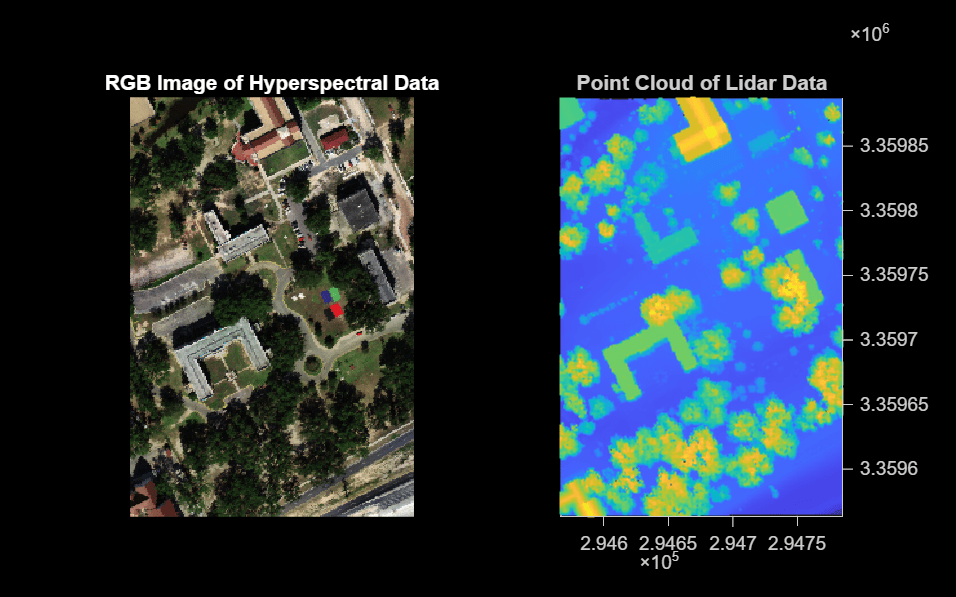
This example uses data from the MUUFL Gulfport Data Set [1][2]. The MUUFL Gulfport Data Set consists of data acquired simultaneously by airborne hyperspectral and lidar sensors mounted on an aircraft over the University of Southern Mississippi – Gulfport in November 2010. The data was acquired using an integrated system that included a hyperspectral sensor to collect hyperspectral data, a lidar sensor to collect lidar data, and a navigation system to collect latitude and longitude data. Because the hyperspectral and lidar data were acquired simultaneously, they are already spatially registered, and there is one-to-one mapping between the pixels of the hyperspectral image and the points in the lidar point cloud. Additionally, the data collected from the navigation system contains latitude and longitude world coordinates for each pixel in the hyperspectral image, and consequently for each point in the aerial point cloud.

Download and unzip the data set.

zipFile = matlab.internal.examples.downloadSupportFile("image","data/gulfport_dataset.zip");
[filepath,folder,~] = fileparts(zipFile);
unzip(zipFile,filepath)

Load Hyperspectral and Lidar Data

Load the hyperspectral data into the workspace as a hypercube object.

filename = fullfile(filepath,folder,"gulfport_dataset","hyperspectralData.dat");
hcube = hypercube(filename);
rows = hcube.Metadata.Height;
cols = hcube.Metadata.Width;

Generate an RGB composite image from the hyperspectral data.

rgbImg = colorize(hcube,Method="rgb",ContrastStretching=true);

Load the lidar data into the workspace as a lasFileReader (Lidar Toolbox) object, and read the point cloud from the lidar data.

filename = fullfile(filepath,folder,"gulfport_dataset","lidarData.las");
lasReader = lasFileReader(filename);
ptCloud = readPointCloud(lasReader);

Display the RGB image derived from hyperspectral data to visualize the scene. Also, display the elevation map of lidar data. Elevation map represents the elevations of points within the point cloud, projected onto the xy-plane.

figure(Units="normalized",Position=[0 0 0.5 0.5])
tiledlayout(1,2)
nexttile
imshow(rgbImg)
axis equal tight
title("RGB Image of Hyperspectral Data",Color="white")
nexttile
pcshow(ptCloud.Location,ViewPlane="XY")
title("Point Cloud of Lidar Data")

Detect Trees and Buildings

Select Seed Pixels

To detect different regions in the scene, you must specify seed pixels to be used for region detection. The scene used for this example contains two distinct regions: vegetation and manmade structure. The vegetation region includes trees and grass. The manmade structures include buildings and roads. You can select the seed pixels for region detection using one of these methods.

useInteractiveROI = false;
numberOfVegetationPoints = 2;
numberOfInfrastructurePoints = 2;
if useInteractiveROI
    [vegetationPoints,infrastructurePoints] = helperSelectSeedPoints(numberOfVegetationPoints,numberOfInfrastructurePoints,rgbImg);
else
    vegetationPoints = [225 121; 50 33];
    infrastructurePoints = [311 18; 182 84];
end

Detect Vegetation and Manmade Structures

Compute the average spectra of the identified tree pixels and the identified building pixels, respectively, as reference.

vegetationRef = [];
infrastructureRef = [];
for i = 1:size(vegetationPoints,1)
    loc = vegetationPoints(i,:);
    pt = squeeze(hcube.DataCube(loc(1),loc(2),:));
    vegetationRef = [vegetationRef pt];
end
for i = 1:size(infrastructurePoints,1)
    loc = infrastructurePoints(i,:);
    pt = squeeze(hcube.DataCube(loc(1),loc(2),:));
    infrastructureRef = [infrastructureRef pt];
end
vegetationRef = mean(vegetationRef,2);
infrastructureRef = mean(infrastructureRef,2);

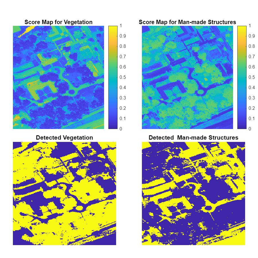
Spectral matching techniques compare individual pixel spectra with a reference spectrum. The spectral angle mapper (SAM) method of spectral matching measures the angle between the reference spectrum and individual pixel spectra. Hence, a lower SAM score is equivalent to a smaller angle between the two spectra, and indicates a higher similarity between the two spectra.

Compute the SAM score between each individual pixel spectrum in the hyperspectral image and the reference spectra for trees and buildings by using the sam function. Threshold the SAM scores using Otsu's method to obtain a mask for trees and buildings. Visualize the masks. Observe that using only spectral information results in classifying all vegetation, including grass, as trees and all manmade structures, including roads, as buildings.

vegetationScore = sam(hcube,vegetationRef);
vegetationMask = vegetationScore <= multithresh(vegetationScore);
infrastructureScore = sam(hcube,infrastructureRef);
infrastructureMask = infrastructureScore <= multithresh(infrastructureScore);
fig = figure(Position=[0.05 0.05 600 600]);
subplot(Position=[0.05 0.5 0.45 0.4],Parent=fig);
imagesc(vegetationScore)
title("Score Map for Vegetation")
axis off
colorbar
clim([0 1])
subplot(Position=[0.55 0.5 0.45 0.4],Parent=fig);
imagesc(infrastructureScore)
title("Score Map for Man-made Structures")
axis off
colorbar
clim([0 1])
subplot(Position=[0.05 0.05 0.4 0.4],Parent=fig);
imagesc(vegetationMask)
title("Detected Vegetation")
axis off
subplot(Position=[0.55 0.05 0.4 0.4],Parent=fig);
imagesc(infrastructureMask)
title("Detected  Man-made Structures")
axis off

Refine Detections to Extract Trees and Buildings

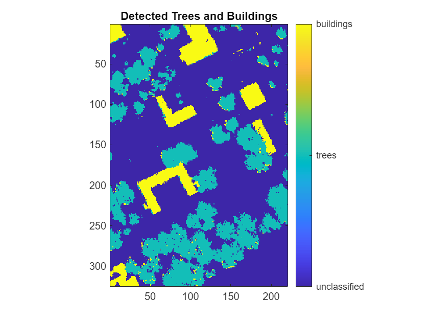
Use the elevation data from the lidar sensor to differentiate between trees and grass and between buildings and roads to get refined masks for trees and buildings, respectively.

elevationData = reshape(ptCloud.Location(:,3),rows,cols);
elevationMask = elevationData;
elevationMask(~vegetationMask & ~infrastructureMask) = 0;
elevationMask = elevationMask >= multithresh(elevationData);
treesMask = vegetationMask & elevationMask;
buildingsMask = infrastructureMask & elevationMask;

Create labels using the masks for trees and buildings.

predictedLabels = zeros(rows,cols);
predictedLabels(treesMask) = 1;
predictedLabels(buildingsMask) = 2;

Create a dictionary to assign a name for each predicted label.

labelNames = ["unclassified" "trees" "buildings"];
labelMap = dictionary(unique(predictedLabels)',labelNames)

labelMap =

  dictionary (double ⟼ string) with 3 entries:

    0 ⟼ "unclassified"
    1 ⟼ "trees"
    2 ⟼ "buildings"

Assign the label names to the predicted labels.

labels = labelMap(predictedLabels);

Visualize the labels.

figure
imagesc(predictedLabels)
axis equal tight
colorbar(Ticks=unique(predictedLabels),TickLabels=labelNames)
title("Detected Trees and Buildings")

Load Geographical Coordinates

Load the world coordinate data into the workspace. This data contains latitude and longitude values, in degrees, for each pixel of the hyperspectral data, and consequently of the lidar data.

filename = fullfile(filepath,folder,"gulfport_dataset","worldCoordinates.mat");
load(filename,"lat","lon")

Create Georeferenced Point Cloud

The loaded latitude and longitude values have a one-to-one mapping with each point in the point cloud captured by the Lidar sensor. However, the point cloud data is currently in a projected coordinate system. To align the point cloud locations with the road network locations obtained from the OpenStreetMap (OSM) web service, you must georeference the point cloud. This involves using the latitude and longitude information to convert the point cloud data into a local coordinate system that matches the geographical coordinates of the road network.

Select the mean values of the latitude, longitude, and altitude to define the georeference point of the point cloud. You can get the altitude from the elevation data in the point cloud. Note that you must use the same georeference origin to download the road network of interest from the OSM web service.

geoReference = [mean(lat(:)) mean(lon(:)) mean(elevationData(:))];

Convert the latitude, longitude, and altitude to the local coordinate system, with geoReference as the origin.

[xE,yN,zU] = latlon2local(lat(:),lon(:),elevationData(:),geoReference);

Create a dictionary to assign a color to each predicted label name.

labelColors = {uint8([0 0 0]),uint8([0 255 0]),uint8([255 0 0])};
colorMap = dictionary(labelNames,labelColors)

colorMap =

  dictionary (string ⟼ cell) with 3 entries:

    "unclassified" ⟼ {[0 0 0]}
    "trees"        ⟼ {[0 255 0]}
    "buildings"    ⟼ {[255 0 0]}

Map the predicted labels of all the points of the scene to the Color property of the point cloud, and create a georeferenced point cloud.

pcColor = cell2mat(colorMap(labels(:)));
georeferencedPointCloud = pointCloud([xE yN zU],Color=pcColor,Intensity=ptCloud.Intensity);

Extract Cuboids of Trees and Buildings from Georeferenced Point Cloud

To generate a RoadRunner Scene containing static objects such as trees and buildings, you must have cuboid parameters that include the center, dimensions, and orientation for each static object. The helperExtractCuboidsFromLidar helper function associates the cuboids with the type of static objects such as trees and buildings, detected using hyperspectral and Lidar data.

Create a parameter structure that contains a field for each type of static object. Specify each static object field as a structure containing these fields:

vegetationParams = struct("minDistance",1.3,"NumClusterPoints",[5 50]);
buildingParams = struct("minDistance",2.5,"NumClusterPoints",50);
parameters = struct(labelNames(2),vegetationParams,labelNames(3),buildingParams);

Obtain the cuboid parameters for each instance of a static object in the point cloud with a specified label from the point cloud by using the helperExtractCuboidsFromLidar helper function. The helper function returns the parameters in a cell array, cuboids.

cuboids = helperExtractCuboidsFromLidar(georeferencedPointCloud,parameters,labelNames(2:3),colorMap);

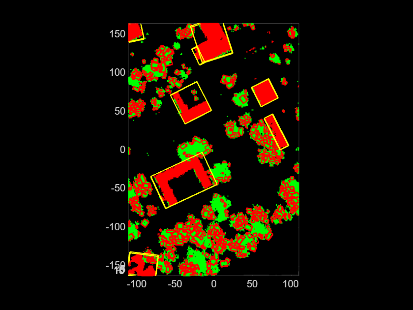
The lidar data used in this example has been recorded by an aerial lidar sensor with a bird's-eye field of view. So, most of the points are on the tops of buildings and trees, with very few on the sides. As a result, the extracted cuboids might not be accurate, and the generated scene might place some objects in the air. To correct this, extend the height of the objects to the ground plane using the addElevation function

numTrees = size(cuboids{1},1);
cuboids = cell2mat(cuboids);
elevationFixedCuboids = addElevation(cuboids,georeferencedPointCloud);
treeCuboids = elevationFixedCuboids(1:numTrees,:);
buildingCuboids = elevationFixedCuboids(numTrees+1:end,:);

Visualize the corrected cuboid parameters overlaid on the point cloud.

ax = pcshow(georeferencedPointCloud,ViewPlane="XY");
hold on
showShape("cuboid",treeCuboids,Color="red",Parent=ax,LineWidth=1)
showShape("cuboid",buildingCuboids,Color="yellow",Parent=ax,LineWidth=1)
hold off

Extract Roads Using OpenStreetMap Web Service

To add the road network into the RoadRunner scene, first download the map file from the OpenStreetMap (OSM) [3] website for the same area that represents the downloaded hyperspectral and lidar data.

Import the OSM road network by using the getMapROI function. Use the geoReference point of the point cloud to get the latitude and longitude values for the OSM road network, and the mean of the limits of the point cloud as extents of the road network.

osmExtent = mean(abs([georeferencedPointCloud.XLimits georeferencedPointCloud.YLimits]));
mapParameters = getMapROI(geoReference(1),geoReference(2),Extent=osmExtent);
osmFileName = websave("RoadScene.osm",mapParameters.osmUrl,weboptions(ContentType="xml"));

Create an empty driving scenario object.

scenario = drivingScenario;

Import the roads obtained from the OpenStreetMap web service into the driving scenario.

roadNetwork(scenario,"OpenStreetMap",osmFileName)

Generate RoadRunner HD Map with Lanes and Static Objects

Create RoadRunner HD Map

Create a RoadRunner HD Map containing the road network imported from the OpenStreetMap web service by using the getRoadRunnerHDMap function.

rrMap = getRoadRunnerHDMap(scenario);

Update Lane Information in RoadRunner HD Map

As the elevation information for the road might not be accurate, improve the road elevation with reference to the point cloud by using the addElevation function.

laneInfo = addElevation(rrMap,georeferencedPointCloud);

Update the RoadRunner HD Map using the road network with improved elevation data.

rrMap.Lanes = laneInfo.Lanes;
rrMap.LaneBoundaries = laneInfo.LaneBoundaries;
rrMap.LaneGroups = laneInfo.LaneGroups;

Update Static Object Information in RoadRunner HD Map

The hyperspectral data used in this example contains a few trees that appear to be placed on roads. Because the hyperspectral image is aerial data and, road-side plant canopies generally occlude the aerial visibility of roads, some parts of roads have been misclassified as trees.

To correct this, remove the misclassified trees from the roads by using the helperRemoveTreesFromRoads helper function, attached to this example as a supporting file.

statObjs.trees = helperRemoveTreesFromRoads(scenario,treeCuboids,georeferencedPointCloud,[rows cols]);

The data in this example contains buildings of different heights. To generate RoadRunner asset paths for buildings based on their heights, use the helperGenerateAssetPaths helper function, attached to this example as a supporting file.

[statObjs.buildings,params.buildings.AssetPath] = helperGenerateAssetPaths("buildings",buildingCuboids);

Generate static object information in the RoadRunner HD Map format by using the roadrunnerStaticObjectInfo function.

objectsInfo = roadrunnerStaticObjectInfo(statObjs,Params=params);

Update the map with the information on the trees and buildings.

rrMap.StaticObjectTypes = objectsInfo.staticObjectTypes;
rrMap.StaticObjects = objectsInfo.staticObjects;

Visualize and Write RoadRunner HD Map

Plot the map, which contains information for the static objects, lane boundaries, and lane centers.

f = figure(Position=[1000 818 700 500]);
ax = axes("Parent",f);
plot(rrMap,ShowStaticObjects=true,Parent=ax)
xlim([-100 100])
ylim([-180 180])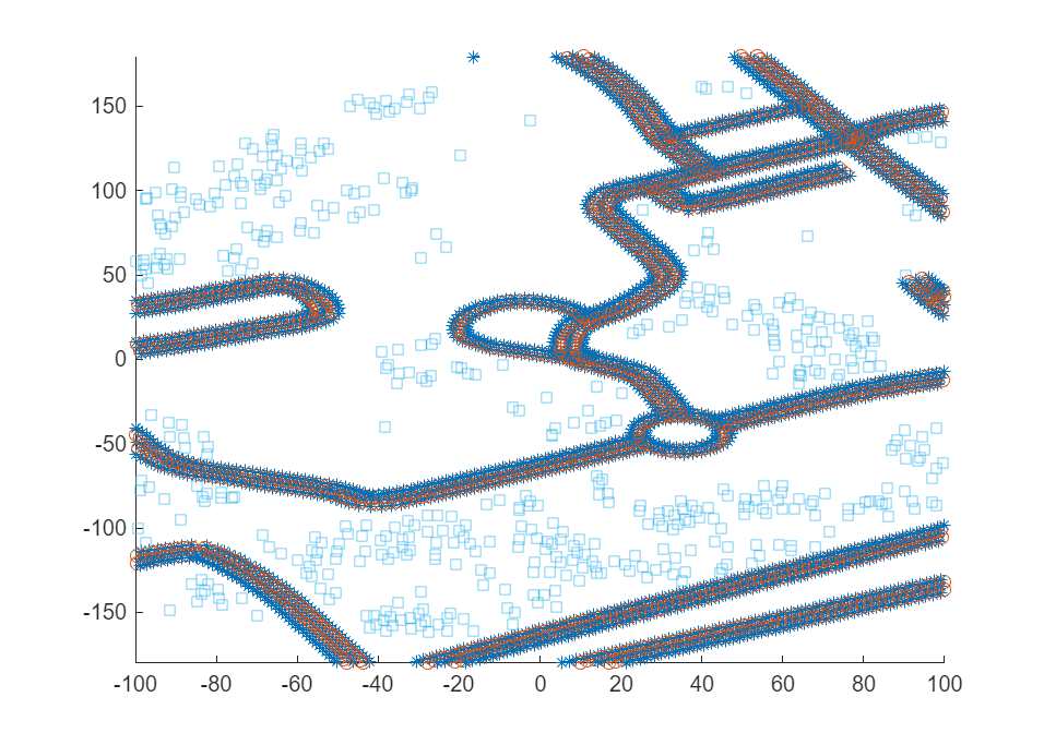

Write the RoadRunner HD Map to a binary file in the present working directory, which you can import into the Scene Builder Tool.

rrMapFileName = "RoadRunnerAerialScene.rrhd";
write(rrMap,rrMapFileName)

Build and Import Scene Using RoadRunner

Open the RoadRunner application by using the roadrunner (RoadRunner) object. Import the RoadRunner HD Map data from your binary file, and build it in the currently open scene.

Specify the path to your local RoadRunner installation folder. This code shows the path for the default installation location on Windows®. For information about creating a project in RoadRunner, see RoadRunner Project and Scene System (RoadRunner).

rrAppPath = "C:\Program Files\RoadRunner " + matlabRelease.Release + "\bin\win64";

Specify the path to your RoadRunner project. This code shows the path to a sample project folder on Windows.

rrProjectPath = "C:\RR\MyProject";

Open RoadRunner using the specified path to your project.

rrApp = roadrunner(rrProjectPath,InstallationFolder=rrAppPath);

Copy the RoadRunnerAerialScene.rrhd scene file into the Assets folder of the RoadRunner project, and import it into RoadRunner.

copyfile(rrMapFileName,(rrProjectPath + filesep + "Assets"));
rrhdFile = fullfile(rrProjectPath,"Assets",rrMapFileName);

Clear the overlap groups option to enable RoadRunner to create automatic junctions at the geometric overlaps of the roads.

enableOverlapGroupsOpts = enableOverlapGroupsOptions(IsEnabled=0);
buildOpts = roadrunnerHDMapBuildOptions(EnableOverlapGroupsOptions=enableOverlapGroupsOpts);
importOptions = roadrunnerHDMapImportOptions(BuildOptions=buildOpts);

Import the scene into RoadRunner by using the importScene function.

importScene(rrApp,rrhdFile,"RoadRunner HD Map",importOptions)

Note: Use of the Scene Builder Tool requires a RoadRunner Scene Builder license, and use of RoadRunner Assets requires a RoadRunner Asset Library Add-On license.

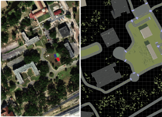
This figure shows the RGB image of the hyperspectral data, and the RoadRunner Scene built using RoadRunner Scene Builder.

References

[1] P. Gader, A. Zare, R. Close, J. Aitken, and G. Tuell. “MUUFL Gulfport Hyperspectral and LiDAR Airborne Data Set.” Technical Report REP-2013-570. University of Florida, Gainesville, 2013. https://github.com/GatorSense/MUUFLGulfport/tree/master.

[2] X. Du and A. Zare. “Technical Report: Scene Label Ground Truth Map for MUUFL Gulfport Data Set.” University of Florida, Gainesville, 2017. https://ufdc.ufl.edu/IR00009711/00001.

[3] You can download OpenStreetMap files from https://www.openstreetmap.org, which provides access to crowd-sourced map data all over the world. The data is licensed under the Open Data Commons Open Database License (ODbL), https://opendatacommons.org/licenses/odbl/.