tune

Tune Bayesian nonlinear non-Gaussian state-space model posterior sampler

Since R2024b

Syntax

[params,Proposal] = tune(PriorMdl,Y,params0)

[params,Proposal] = tune(PriorMdl,Y,params0,Name=Value)

Description

The Markov chain Monte Carlo (MCMC) method used by the simulate function to sample from the posterior distribution requires a carefully specified proposal distribution. You can use the tune function to search for an adequate posterior mode for simulate, to improve the proposal distribution, and therefore, the acceptance rate of the proposed posterior draws.

[params,Proposal] = tune(PriorMdl,Y,params0) returns optimized proposal distribution parameter mean vector params and scale matrix Proposal to improve the MCMC sampler used by simulate. PriorMdl is the Bayesian nonlinear non-Gaussian state-space model that specifies the state-space model structure (likelihood) and prior distribution, Y is the data for the likelihood, and params0 is the vector of initial values for the unknown state-space model parameters Θ in PriorMdl.

example

[params,Proposal] = tune(PriorMdl,Y,params0,Name=Value) specifies additional options using one or more name-value arguments. For example, tune(PriorMdl,Y,params0,Hessian="opg",Display="off") uses the outer-product of gradients method to compute the Hessian matrix and suppresses the display of the optimized values.

example

Examples

collapse all

Tune Proposal Distribution for MCMC Sampler

Open Live Script

Simulate observed responses from a known nonlinear state-space model, then treat the model as Bayesian and draw parameters from the posterior distribution. Tune the proposal distribution of the MCMC sampler by using tune.

Consider this data-generating process (DGP).

$\begin{array}{l} x_{t} = 0.7 x_{t - 1} + \sqrt{0.2} u_{t} \\ y_{t} \sim P o i s s o n (3 e^{x_{t}}), \end{array}$

where the series $u_{t}$ is a standard Gaussian series of random variables.

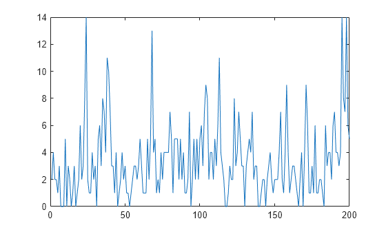
Simulate a series of 200 observations from the process.

rng(1,"twister")    % For reproducibility
T = 200;
thetaDGP = [0.7; 0.2; 3];

numparams = numel(thetaDGP);

MdlXSim = arima(AR=thetaDGP(1),Variance=thetaDGP(2), ...
    Constant=0);
xsim = simulate(MdlXSim,T);
y = random("poisson",thetaDGP(3)*exp(xsim));

figure
plot(y)

Figure contains an axes object. The axes object contains an object of type line.

Suppose the structure of the DGP is known, but the model parameters trueTheta are unknown, explicitly

$\begin{array}{l} x_{t} = ϕ x_{t - 1} + σ u_{t} \\ y_{t} \sim P o i s s o n (λ e^{x_{t}}), \end{array}$

Consider a Bayesian nonlinear non-Gaussian state-space model representing the unknown parameters. Assume that the prior distributions are:

$ϕ \sim N_{(- 1, 1)} (m_{0}, v_{0}^{2})$ , that is, a truncated normal distribution with $ϕ \in [- 1, 1]$ .
$σ^{2} \sim IG (a_{0}, b_{0})$ , that is, an inverse gamma distribution with shape $a_{0}$ and scale $b_{0}$ .
$λ \sim Gamma (α_{0}, β_{0})$ , that is, a gamma distribution with shape $α_{0}$ and scale $β_{0}$ .

The Local Functions section contains the functions paramMap and priorDistribution required to specify the Bayesian nonlinear state-space model. The paramMap function specifies the state-space model structure and initial state moments. The priorDistribution function returns the log of the joint prior distribution of the state-space model parameters. You can use the functions only within this script.

Create a Bayesian nonlinear state-space model for the DGP.

Arbitrarily choose values for the hyperparameters.
Indicate that the state-space model observation equation is expressed as a distribution.
To speed up computations, the arguments A and LogY of the paramMap function are written to enable simultaneous evaluation of the transition and observation densities of multiple particles. Specify this characteristic by using the Multipoint name-value argument.

% pi(phi,sigma2) hyperparameters
m0 = 0;                 
v02 = 1;
a0 = 1;
b0 = 1;

% pi(lambda) hyperparameters
alpha0 = 3;
beta0 = 1;

hyperparams = [m0 v02 a0 b0 alpha0 beta0];

PriorMdl = bnlssm(@paramMap,@(x)priorDistribution(x,hyperparams), ...
    ObservationForm="distribution",Multipoint=["A" "LogY"]);

PriorMdl is a bnlssm model specifying the state-space model structure and prior distribution of the state-space model parameters. Because PriorMdl contains unknown values, it serves as a template for posterior estimation with observations.

The simulate function requires a proposal distribution scale matrix. You can obtain a data-driven proposal scale matrix by using the tune function. Alternatively, you can supply your own scale matrix.

Obtain a data-driven scale matrix by using the tune function. Supply an arbitrarily chosen set of initial parameter values.

theta0 = [0.5; 0.1; 2]; 
[theta0,Proposal] = tune(PriorMdl,y,theta0)

         Optimization and Tuning        
      | Params0  Optimized  ProposalStd 
----------------------------------------
 c(1) |  0.5000    0.6081      0.0922   
 c(2) |  0.1000    0.2190      0.0503   
 c(3) |   2        2.8497      0.2918

theta0 = 3×1

    0.6081
    0.2190
    2.8497

Proposal = 3×3

    0.0085   -0.0026    0.0033
   -0.0026    0.0025   -0.0040
    0.0033   -0.0040    0.0852

theta0 is a 3-by-1 estimate of the posterior mode and Proposal is the corresponding Hessian matrix. Both outputs are the optimized moments of the proposal distribution, the latter of which is up to a proportionality constant. tune displays convergence information and an estimation table, which you can suppress by using the Display options of the optimizer and tune.

Draw 1000 random parameter vectors from the posterior distribution. Specify the simulated response path as observed responses and the optimized values returned by tune for the initial parameter values and the proposal distribution.

[Theta,accept] = simulate(PriorMdl,y,theta0,Proposal);
accept

accept = 
0.4210

Theta is a 3-by-1000 matrix of randomly drawn parameters from the posterior distribution. Rows correspond to the elements of the input argument theta of the functions paramMap and priorDistribution.

accept is the proposal acceptance probability. In this case, simulate accepts 42% of the proposal draws.

Plot trace plots of the posterior sample.

paramnames = ["\phi" "\sigma^2" "\lambda"];

figure
h = tiledlayout(3,1);
for j = 1:numparams
    nexttile
    plot(Theta(j,:))
    hold on
    yline(thetaDGP(j))
    ylabel(paramnames(j))
end
title(h,"Posterior Trace Plots")

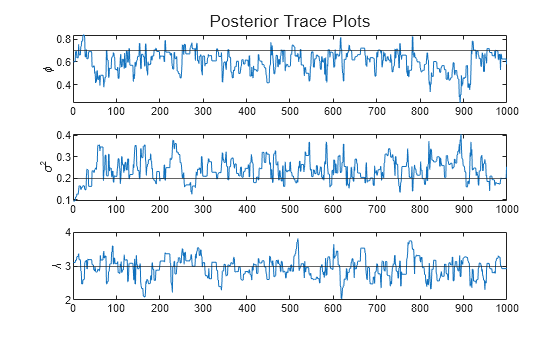
$Figure contains 3 axes objects. Axes object 1 with ylabel \phi contains 2 objects of type line, constantline. Axes object 2 with ylabel \sigma^2 contains 2 objects of type line, constantline. Axes object 3 with ylabel \lambda contains 2 objects of type line, constantline.$

The sampler eventually settles at near the true values of the parameters. In this case, the sample shows serial correlation and transient behavior. You can remedy serial correlation in the sample by adjusting the Thin name-value argument, and you can remedy transient effects by increasing the burn-in period using the BurnIn name-value argument.

Local Functions

These functions specify the state-space model parameter mappings, in distribution form, and the log prior distribution of the parameters.

function [A,B,LogY,Mean0,Cov0,StateType] = paramMap(theta)
    A = theta(1); 
    B = sqrt(theta(2));
    LogY = @(y,x)y.*(x + log(theta(3)))- exp(x).*theta(3);
    Mean0 = 0;
    Cov0 = 2;
    StateType = 0;     % Stationary state process
end

function logprior = priorDistribution(theta,hyperparams)
    % Prior of phi
    m0 = hyperparams(1);
    v20 = hyperparams(2);
    pphi = makedist("normal",mu=m0,sigma=sqrt(v20));
    pphi = truncate(pphi,-1,1);
    lpphi = log(pdf(pphi,theta(1)));

    % Prior of sigma2
    a0 = hyperparams(3);
    b0 = hyperparams(4);
    lpsigma2 = -a0*log(b0) - log(gamma(a0)) + (-a0-1)*log(theta(2)) - ...
        1./(b0*theta(2));

    % Prior of lambda
    alpha0 = hyperparams(5);
    beta0 = hyperparams(6);
    plambda = makedist("gamma",alpha0,beta0);
    lplambda = log(pdf(plambda,theta(3))); 

    logprior = lpphi + lpsigma2 + lplambda;
end

Adjust Proposal Tuning Algorithm

Open Live Script

Adjust the tuning algorithm that obtains optimal proposal moments for the MCMC sampler used to draw posterior samples from a Bayesian nonlinear stochastic volatility model. The response series is daily S&P 500 closing returns. For a full exposition of this problem, see Fit Bayesian Stochastic Volatility Model to S&P 500 Volatility.

Load the data set Data_GlobalIdx1.mat, and then extract the S&P 500 closing prices (last column of the matrix Data).

load Data_GlobalIdx1
sp500 = Data(:,end);
T = numel(sp500);
dts = datetime(dates,ConvertFrom="datenum");

Convert the price series to returns, and then center the returns.

retsp500 = price2ret(sp500);
y = retsp500 - mean(retsp500);
retdts = dts(2:end);

Consider the nonlinear state-space form of the stochastic volatility model for observed asset returns $y_{t}$ :

$\begin{array}{l} x_{t + Δ t} = α + β x_{t} + σ u_{t} \\ y_{t} = e x p (\frac{1}{2} x_{t}) \sqrt{Δ t} ε_{t}, \end{array}$

where:

$Δ t = \frac{1}{365}$ for daily returns.
$x_{t}$ is a latent AR(1) process representing the conditional volatility series.
$u_{t}$ are $ε_{t}$ are mutually independent and individually iid random standard Gaussian noise series.

The linear state-space coefficient matrices are:

$A = [\begin{array}{c} β & α \\ 0 & 1 \end{array}] .$
$B = [\begin{array}{c} σ \\ 0 \end{array}] .$

The observation equation is nonlinear. Because $ε_{t}$ is a standard Gaussian random variable, the conditional distribution of $y_{t}$ given $x_{t}$ and the parameters is Gaussian with a mean of 0 and standard deviation $\sqrt{Δ t} \exp (0.5 x_{t})$ .

The local function paramMap, which uses the distribution form for the observation equation, specifies this model structure. Unlike the parameter mapping function in Fit Bayesian Stochastic Volatility Model to S&P 500 Volatility, paramMap reduces the number of states to one for computational efficiency.

Assume a flat prior, that is, the log prior is 0 over the support of the parameters and -Inf everywhere else. The local function flatLogPrior specifies the prior.

Create a Bayesian nonlinear state-space model that specifies the model structure and prior distribution. Specify that the observation equation is in distribution form and that bnlssm functions can evaluate multiple particles simultaneously for A and LogY.

PriorMdl = bnlssm(@paramMap,@flatLogPrior,ObservationForm="distribution", ...
    Multipoint=["A" "LogY"]);

Tune the proposal distribution. Specify an arbitrarily chosen set of initial parameter values and the following settings:

Set the search interval for $β$ to (-1,1). Specified search intervals apply only to tuning the proposal.
Set the search interval for $σ$ to (0, $\infty$ ).
Specify computing the Hessian by the outer product of gradients.
For computational speed, do not sort the particles by using Hilbert sorting.

theta0 = [0.2 0 0.5];
lower = [-1; -Inf; 0];
upper = [1; Inf; Inf];
rng(1)

[params,Proposal] = tune(PriorMdl,y,theta0,Lower=lower,Upper=upper, ...
    NumParticles=500,Hessian="opg",SortParticles=false);

         Optimization and Tuning        
      | Params0  Optimized  ProposalStd 
----------------------------------------
 c(1) |  0.2000    0.9949      0.0030   
 c(2) |   0       -0.0155      0.0116   
 c(3) |  0.5000    0.1495      0.0130

Obtain a sample from the posterior distribution. Specify the optimal proposal a burn-in period of 1e4 and retain every 25th draw to reduce serial correlation among the draws. The sampler, with these settings, takes some time to complete.

burnin = 1e4;
thin = 25;

[ThetaPost,accept] = simulate(PriorMdl,y,params,Proposal, ...
    BurnIn=burnin,Thin=thin);
accept

accept = 
0.5131

Determine the quality of the posterior sample by plotting trace plots of the parameter draws.

figure
plot(ThetaPost(1,:))
title("Trace Plot: \beta")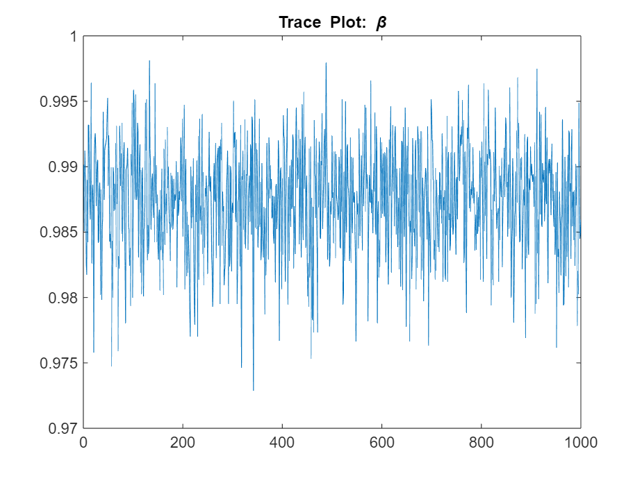

figure
plot(ThetaPost(2,:))
title("Trace Plot: \alpha")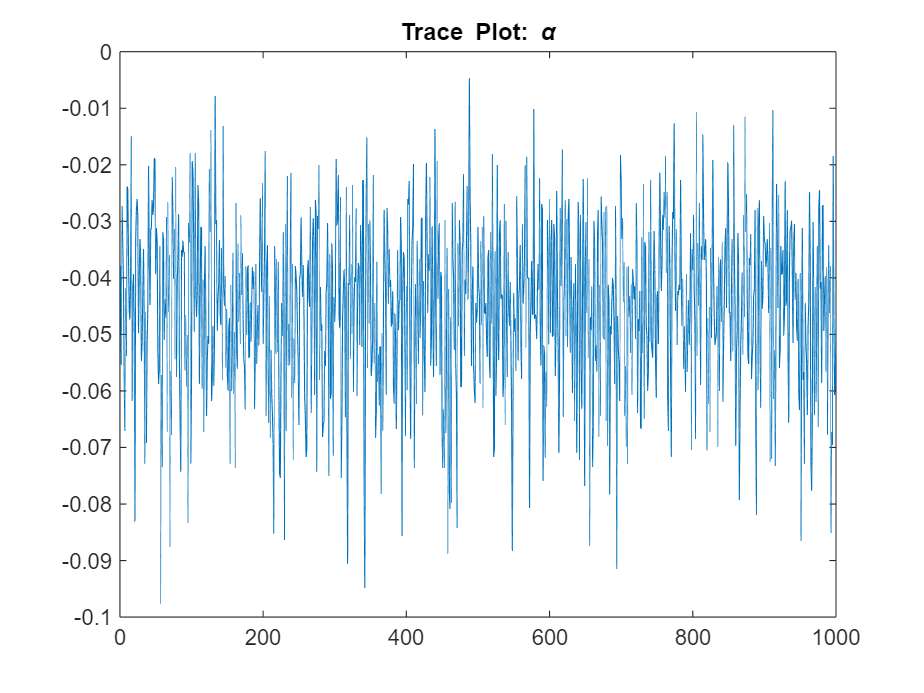

figure
plot(ThetaPost(3,:))
title("Trace Plot: \sigma")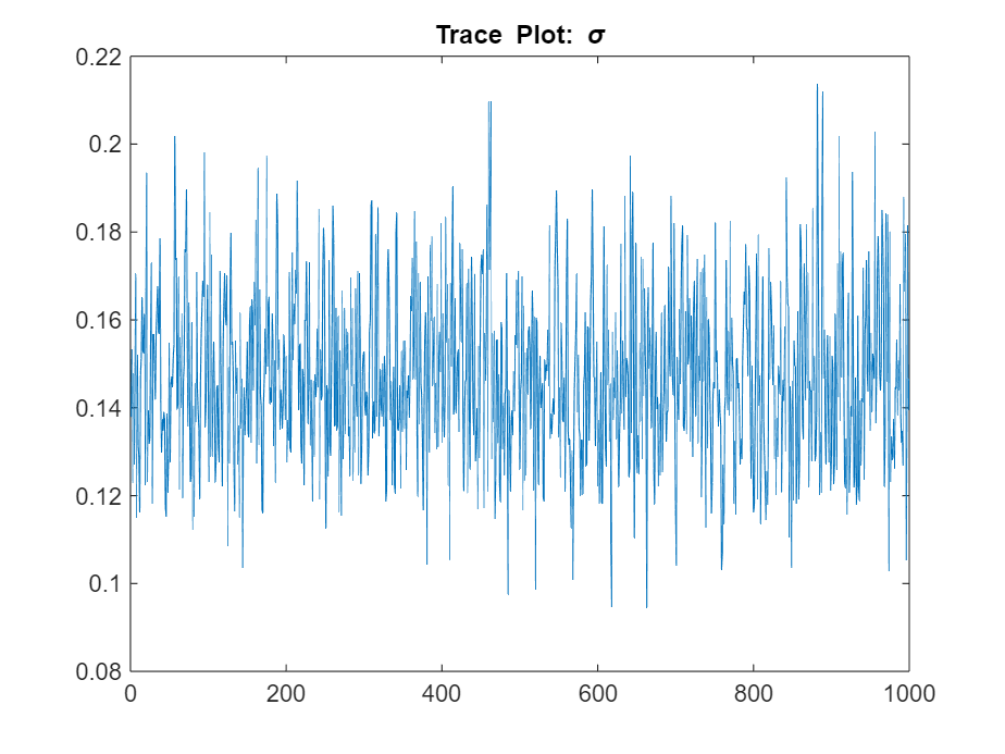

The posterior samples show good mixing with some minor serial correlation.

Local Functions

This example uses the following functions. paramMap is the parameter-to-matrix mapping function and flatLogPrior is the log prior distribution of the parameters.

function [A,B,LogY,Mean0,Cov0,StateType] = paramMap(theta)
    A = @(x) theta(2) + theta(1).*x;
    B = theta(3);
    LogY = @(y,x)-0.5.*x-0.5*365*y*y.*exp(-x);
    Mean0 = theta(2)./(1 - theta(1));          
    Cov0 = (theta(3)^2)./(1 - theta(1)^2);
    StateType = 0;
end

function logprior = flatLogPrior(theta)
% flatLogPrior computes the log of the flat prior density for the three
% variables in theta. Log probabilities for parameters outside the
% parameter space are -Inf.
    paramcon = zeros(numel(theta),1);
    % theta(1) is the lag 1 term in a stationary AR(1) model. The
    % value needs to be within the unit circle.
    paramcon(1) = abs(theta(1)) >= 1 - eps;

    % alpha must be finite
    paramcon(2) = ~isfinite(theta(2)); 

    % Standard deviation of the state disturbance theta(3) must be positive.
    paramcon(3) = theta(3) <= eps;

    if sum(paramcon) > 0
        logprior = -Inf;
    else
        logprior = 0;   % Prior density is proportional to 1 for all values
                        % in the parameter space.
    end
end

Compare SMC Proposal Methods

Open Live Script

This example compares the performance of several SMC proposal particle resampling methods for obtaining random paths of parameter values from the posterior distribution of a quasi-nonnegative constrained state space model, which models nonnegative state quantities such as interest rates and prices:

$\begin{array}{l} x_{t} = \max (0, a_{0} + a_{1} x_{t - 1}) + b u_{t} \\ y_{t} = x_{t} + d ε_{t} . \end{array}$

$u_{t}$ and $ε_{t}$ are iid standard Gaussian random variables.

Generate Artificial Data

Consider the following data-generating process (DGP)

$\begin{array}{l} x_{t} = \max (0, 0.1 + 0.95 x_{t - 1}) + u_{t} \\ y_{t} = x_{t} + 0.5 ε_{t} . \end{array}$

Generate a random series of 200 observations from the DGP.

a0 = 0.1;
a1 = 0.95;
b = 1;
d = 0.5;
theta = [a0; a1; b; d];
T = 200;

% Preallocate variables
x = zeros(T,1);
y = zeros(T,1);

rng(0,"twister") % For reproducibility
u = randn(T,1);
e = randn(T,1);

for t = 2:T
    x(t) = max(0,a0 + a1*x(t-1)) + b*u(t);
    y(t) = x(t) + d*e(t);               
end

Create Bayesian Nonlinear State-Space Model

The Local Functions section contains two functions required to specify the Bayesian nonlinear state-space model: the state-space model parameter mapping function paramMap and the prior distribution of the parameters priorDistribution. You can use the functions only within this script.

The paramMap function has these qualities:

Functions can simultaneously evaluate the state equation for multiple values of A. Therefore, you can speed up calculations by specifying the Multipoint="A" option.
The observation equation is in equation form, that is, the function composing the states is nonlinear and the innovation series $ε_{t}$ is additive, linear, and Gaussian.

The priorDistribution function specifies a flat prior, which has a density that is proportional to 1 everywhere in the parameter space; it constrains the error standard deviations to be positive.

Create a Bayesian nonlinear state-space model characterized by the system.

PriorMdl = bnlssm(@paramMap,@priorDistribution,Multipoint="A");

Draw Random Parameter Paths from Posterior Using Each Proposal Sampler Method

Obtain random parameter paths from the joint posterior distribution using the bootstrap, optimal, and one-pass unscented particle resampling methods. Tune the sampler initialized from a randomly drawn set of values in [0,1], thin the sample by a factor of 10, specify a burn-in period of 100, and draw 1000 paths.

numDraws = 1000;
smcMethod = ["bootstrap" "optimal" "unscented"];
for j = 3:-1:1 % Set last element first to preallocate entire cell vector
    params0 = rand(4,1);
    [params,Proposal] = tune(PriorMdl,y,params0,Display="off",NewSamples=smcMethod(j));
    thetaSim{j} = simulate(PriorMdl,y,params,Proposal,NewSamples=smcMethod(j), ...
        NumDraws=numDraws,Thin=10,Burnin=100);
end

Separately for each parameter, draw histograms of the posterior draws for each method on the same plot.

figure
tiledlayout(2,2)
varnames = ["a0" "a1" "b" "d"];
for j = 1:numel(theta)
    nexttile
    h1 = histogram(thetaSim{1}(j,:));
    hold on
    h2 = histogram(thetaSim{2}(j,:));
    h3 = histogram(thetaSim{3}(j,:));
    h4 = xline(theta(j),"--",LineWidth=2);
    hold off
    title(varnames(j))
end
legend([h1 h2 h3 h4],[smcMethod "True"])

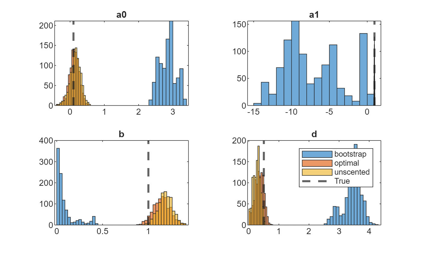
In this case, the optimal and one-pass unscented methods yield distributions closer to the true values than the bootstrap method.

Local Functions

These functions specify the state-space model parameter mappings, in equation form, and log prior distribution of the parameters.

function [A,B,C,D,mean0,Cov0] = paramMap(params)
    a0 = params(1);
    a1 = params(2);
    b = params(3);
    d = params(4);
    A = @(x) max(0,a0+a1.*x);
    B = b;
    C = 1;
    D = d;
    mean0 = 0;
    Cov0 = 1;
end

function logprior = priorDistribution(theta)
    paramconstraints = theta(3:4) <= 0; % b and d are greater than 0
    if(sum(paramconstraints))
        logprior = -Inf;
    else 
        logprior = 0;   % Prior density is proportional to 1 for all values
                        % in the parameter space.
    end
end

Input Arguments

collapse all

`PriorMdl` — Prior Bayesian nonlinear non-Gaussian state-space model
`bnlssm` model object

Prior Bayesian nonlinear non-Gaussian state-space model, specified as a bnlssm model object return by bnlssm.

The function handles of the properties PriorMdl.ParamDistribution and PriorMdl.ParamMap determine the prior and the data likelihood, respectively.

`Y` — Observed response data
numeric matrix | cell vector of numeric vectors

Observed response data, specified as a numeric matrix or a cell vector of numeric vectors.

If PriorMdl is time invariant with respect to the observation equation, Y is a T-by-n matrix. Each row of the matrix corresponds to a period and each column corresponds to a particular observation in the model. T is the sample size and n is the number of observations per period. The last row of Y contains the latest observations.
If PriorMdl is time varying with respect to the observation equation, Y is a T-by-1 cell vector. Y{t} contains an n_t-dimensional vector of observations for period t, where t = 1, ..., T. For linear observation models, the corresponding dimensions of the coefficient matrices, outputs of PriorMdl.ParamMap, C{t}, and D{t} must be consistent with the matrix in Y{t} for all periods. For nonlinear observation models, the dimensions of the inputs and outputs associated with the observations must be consistent. Regardless of model type, the last cell of Y contains the latest observations.

NaN elements indicate missing observations. For details on how tune accommodates missing observations, see Algorithms.

Data Types: double | cell

`params0` — Initial values for parameters Θ
numeric vector

Initial parameter values for the parameters Θ, specified as a numParams-by-1 numeric vector. Elements of params0 must correspond to the elements of the first input arguments of PriorMdl.ParamMap and PriorMdl.ParamDistribution.

Data Types: double

Name-Value Arguments

collapse all

Specify optional pairs of arguments as Name1=Value1,...,NameN=ValueN, where Name is the argument name and Value is the corresponding value. Name-value arguments must appear after other arguments, but the order of the pairs does not matter.

Example: tune(PriorMdl,Y,params0,Hessian="opg",Display="off") uses the outer-product of gradients method to compute the Hessian matrix and suppresses the display of the optimized values.

`NumParticles` — Number of particles
`1000` (default) | positive integer

Number of particles for SMC, specified as a positive integer.

Example: NumParticles=1e4

Data Types: double

`NewSamples` — SMC proposal distribution
`"bootstrap"` (default) | `"optimal"` | `"unscented"` | character vector

Since R2025a

SMC proposal (importance) distribution, specified as a value in this table.

Value SMC Sampler Description

Value	SMC Sampler	Description
`"bootstrap"`	Bootstrap forward filter [7]	SMC samples particles form the state transition distribution (observations do not inform the sampler). This option is available only for models with observation noise (nonzero `D`). This method has a relatively low computational cost, but it does not inform the routine of the current observations, which can increase the Monte Carlo sampling variance.
`"optimal"`	Conditionally optimal proposal [4]	SMC samples particles from the one-step filtering distribution with incremental weights proportional to the likelihood (observations inform the sampler). The weights have minimum variance. This option is available for the following tractable models supplied in equation form: Nonlinear state transition equation and a linear measurement equation Nonlinear model with deterministic state transition equation (`B = 0`)
`"unscented"`	Unscented transformation [11]	SMC proposal distribution is the one-step filtering distribution approximated by the unscented transformation (observations inform the sampler). This option is available only for models in equation form with observation noise (nonzero `D`). By default, this option uses the filtered state mean as the representative point, around which the algorithm generates sigma points. To specify all particles as representative points for the unscented transformation, set `MultiPassUnscented=true`. This setting provides a higher-quality proposal, but it is more computationally expensive.

"bootstrap"

Bootstrap forward filter [7]

SMC samples particles form the state transition distribution (observations do not inform the sampler).

This option is available only for models with observation noise (nonzero D).

This method has a relatively low computational cost, but it does not inform the routine of the current observations, which can increase the Monte Carlo sampling variance.

"optimal"

Conditionally optimal proposal [4]

SMC samples particles from the one-step filtering distribution with incremental weights proportional to the likelihood (observations inform the sampler). The weights have minimum variance.

This option is available for the following tractable models supplied in equation form:

Nonlinear state transition equation and a linear measurement equation
Nonlinear model with deterministic state transition equation (B = 0)

"unscented"

Unscented transformation [11]

SMC proposal distribution is the one-step filtering distribution approximated by the unscented transformation (observations inform the sampler).

This option is available only for models in equation form with observation noise (nonzero D).

By default, this option uses the filtered state mean as the representative point, around which the algorithm generates sigma points. To specify all particles as representative points for the unscented transformation, set MultiPassUnscented=true. This setting provides a higher-quality proposal, but it is more computationally expensive.

Example: NewSamples="unscented"

Data Types: char | string

`MultiPassUnscented` — Flag to apply unscented transformation to all particles
`false` (default) | `true`

Since R2025a

Flag to apply unscented transformation to all particles, specified as a value in this table.

Value Description

Value	Description
`false`	The filtered state mean is the representative point, around which the algorithm generates sigma points. This option is less computationally expensive than `MultiPassUnscented=true`, but it can yield a lower-quality proposal distribution.
`true`	All particles are the representative points. This option is more computationally expensive than the default, but it can yield a higher-quality proposal distribution.

false

The filtered state mean is the representative point, around which the algorithm generates sigma points.

This option is less computationally expensive than MultiPassUnscented=true, but it can yield a lower-quality proposal distribution.

true

All particles are the representative points.

This option is more computationally expensive than the default, but it can yield a higher-quality proposal distribution.

Example: MultiPassUnscented=false

Data Types: logical

`NumPaths` — Number of sample state paths
`200` (default) | positive integer

Number of sample state paths to draw from the posterior smoothed state distribution, specified as a positive integer.

Example: NumPaths=1e4

Data Types: double

`Resample` — SMC resampling method
`"multinomial"` (default) | `"residual"` | `"systematic"`

SMC resampling method, specified as a value in this table.

Value	Description
`"multinomial"`	At time t, the set of previously generated particles (parent set) follows a standard multinomial distribution, with probabilities proportional to their weights. An offspring set is resampled with replacement from the parent set [1].
`"residual"`	Residual sampling, a modified version of multinomial resampling that can produce an estimator with lower variance than the multinomial resampling method [9].
`"systematic"`	Systematic sampling, which produces an estimator with lower variance than the multinomial resampling method [3].

Resampling methods downsample insignificant particles to achieve a smaller estimator variance than if no resampling is performed and to avoid sampling from a degenerate proposal [5].

Example: Resample="residual"

Data Types: char | string

`Cutoff` — Effective sample size threshold for resampling
`0.5*NumParticles` (default) | nonnegative scalar

Effective sample size threshold, below which tune resamples particles, specified as a nonnegative scalar. For more details, see [5], Ch. 12.3.3.

Tip

To resample during every period, set Cutoff=numparticles, where numparticles is the value of the NumParticles name-value argument.
To avoid resampling, set Cutoff=0.

Example: Cutoff=0.75*numparticles

Data Types: double

`SortParticles` — Flag for sorting particles before resampling
`true` (default) | `false`

Flag for sorting particles before resampling, specified as a value in this table.

Value	Description
`true`	`tune` sorts the generated particles before resampling them.
`false`	`tune` does not sort the generated particles.

When SortPartiles=true, tune uses Hilbert sorting during the SMC routine to sort the particles. This action can reduce Monte Carlo variation, which is useful when you compare loglikelihoods resulting from evaluating several params arguments that are close to each other [3]. However, the sorting routine requires more computation resources, and can slow down computations, particularly in problems with a high-dimensional state variable.

Example: SortParticles=false

Data Types: logical

`Lower` — Parameter lower bounds
`[]` (default) | numeric vector

Parameter lower bounds when computing the Hessian matrix (see Hessian), specified as a numParams-by-1 numeric vector.

Lower(j) specifies the lower bound of parameter theta(j), the first input argument of PriorMdl.ParamMap and PriorMdl.ParamDistribution.

The default value [] specifies no lower bounds.

Note

Lower does not apply to posterior simulation. To apply parameter constraints on the posterior, code them in the log prior distribution function PriorMdl.ParamDistribution by setting the log prior of values outside the distribution support to -Inf.

Example: Lower=[0 -5 -1e7]

Data Types: double

`Upper` — Parameter upper bounds
`[]` (default) | numeric vector

Parameter lower bounds when computing the Hessian matrix (see Hessian), specified as a numParams-by-1 numeric vector.

Upper(j) specifies the upper bound of parameter theta(j), the first input argument of PriorMdl.ParamMap and PriorMdl.ParamDistribution.

The default value [] specifies no upper bounds.

Note

Upper does not apply to posterior simulation. To apply parameter constraints on the posterior, code them in the log prior distribution function PriorMdl.ParamDistribution by setting the log prior of values outside the distribution support to -Inf.

Example: Upper=[5 100 1e7]

Data Types: double

`Options` — Optimization options
`optimoptions` optimization controller

Optimization options for tuning the proposal distribution, specified as an optimoptions optimization controller. Options replaces default optimization options of the optimizer. For details on altering default values of the optimizer, see the optimization controller optimoptions, the constrained optimization function fmincon, or the unconstrained optimization function fminunc in Optimization Toolbox™.

For example, to change the constraint tolerance to 1e-6, set options = optimoptions(@fmincon,ConstraintTolerance=1e-6,Algorithm="sqp"). Then, pass Options by using Options=options.

By default, tune uses the default options of the optimizer.

`StepSizeFirstDerivative` — Step size for computing first derivatives
`1e-6` (default) | positive scalar

Step size for computing the first derivatives that comprise the Hessian matrix (see Hessian), specified as a positive scalar.

Example: StepSizeFirstDerivative=1e-4

Data Types: double

`StepSizeSecondDerivative` — Step size for computing second derivatives
`1e-4` (default) | positive scalar

Step size for computing the second derivatives that comprise the Hessian matrix (see Hessian), specified as a positive scalar.

Example: StepSizeSecondDerivative=1e-3

Data Types: double

`Hessian` — Hessian approximation method
`"difference"` (default) | `"diagonal"` | `"opg"` | character vector

Hessian approximation method for the MH proposal distribution scale matrix, specified as a value in this table.

Value	Description
`"difference"`	Finite differencing
`"diagonal"`	Diagonalized result of finite differencing
`"opg"`	Outer product of gradients, ignoring the prior distribution

Tip

The Hessian="difference" setting can be computationally intensive and inaccurate, and the resulting scale matrix can be nonnegative definite. Try one of the other options for better results.

Example: Hessian="opg"

Data Types: char | string

`Display` — Control for displaying proposal-tuning results
`"summary"` (default) | `"full"` | `"off"` | character vector

Control for displaying the proposal-tuning results, specified as a value in this table.

Value	Description
`"off"`	Suppress all output.
`"summary"`	Display a summary of proposal-tuning results.
`"full"`	Display proposal-tuning details.

Example: Display="full"

Data Types: string | char

Output Arguments

collapse all

`params` — Optimized parameter values
numeric vector

Optimized parameter values for the MCMC sampler, returned as a numParams-by-1 numeric vector. params(j) contains the optimized value of parameter theta(j), where theta is the first input argument of PriorMdl.ParamMap and PriorMdl.ParamDistribution.

When you call simulate, pass params as the initial parameter values input params0.

`Proposal` — Proposal distribution covariance/scale matrix
numeric matrix

Proposal distribution covariance/scale matrix for the MCMC sampler, specified as a numParams-by-numParams numeric matrix. Rows and columns of Proposal correspond to elements in params.

Proposal is the scale matrix up to a proportionality constant, which is specified by the Proportion name-value argument of estimate and simulate.

The proposal distribution is multivariate normal or Student's t.

When you call simulate, pass Proposal as the proposal distribution scale matrix input Proposal.

Data Types: double

Tips

Unless you set Cutoff=0, tune resamples particles according to the specified resampling method Resample. Although resampling particles with high weights improves the results of the SMC, you should also allow the sampler traverse the proposal distribution to obtain novel, high-weight particles. To do this, experiment with Cutoff.
Avoid an arbitrary choice of the initial state distribution. bnlssm functions generate the initial particles from the specified initial state distribution, which impacts the performance of the nonlinear filter. If the initial state specification is bad enough, importance weights concentrate on a small number of particles in the first SMC iteration, which might produce unreasonable filtering results. This vulnerability of the nonlinear model behavior contrasts with the stability of the Kalman filter for the linear model, in which the initial state distribution usually has little impact on the filter because the prior is washed out as it processes data.

Algorithms

The MCMC sampler requires a carefully specified proposal distribution. tune tunes the sampler by performing numerical optimization to search for a posterior mode. A reasonable proposal for the multivariate normal or t distribution is the inverse of the negative Hessian matrix, which tune evaluates at the resulting posterior mode.
tune approximates the data likelihood by sequential Monte Carlo (SMC), and it approximates the posterior gradient vector and Hessian matrix by the simulation smoother (simsmooth). tune tunes the sampler by numerical optimization.
When tune tunes the proposal distribution, the optimizer that tune uses to search for a posterior mode before computing the Hessian matrix depends on your specifications.
- tune uses fminunc by default.
- tune uses fmincon when you perform constrained optimization by specifying the Lower or Upper name-value argument.
tune accommodates missing data by not updating filtered state estimates corresponding to missing observations. In other words, suppose there is a missing observation at period t. Then, the state forecast for period t based on the previous t – 1 observations and filtered state for period t are equivalent.

References

[1] Andrieu, Christophe, Arnaud Doucet, and Roman Holenstein. "Particle Markov Chain Monte Carlo Methods." Journal of the Royal Statistical Society Series B: Statistical Methodology 72 (June 2010): 269–342. https://doi.org/10.1111/j.1467-9868.2009.00736.x.

[2] Andrieu, Christophe, and Gareth O. Roberts. "The Pseudo-Marginal Approach for Efficient Monte Carlo Computations." Ann. Statist. 37 (April 2009): 697–725. https://dx.doi.org/10.1214/07-AOS574.

[3] Deligiannidis, George, Arnaud Doucet, and Michael Pitt. "The Correlated Pseudo-Marginal Method." Journal of the Royal Statistical Society, Series B: Statistical Methodology 80 (June 2018): 839–870. https://doi.org/10.1111/rssb.12280.

[4] Doucet, Arnaud, Simon Godsill, and Christophe Andrieu. "On Sequential Monte Carlo Sampling Methods for Bayesian Filtering." Statistics and Computing 10 (July 2000): 197–208. https://doi.org/10.1023/A:1008935410038.

[5] Durbin, J, and Siem Jan Koopman. Time Series Analysis by State Space Methods. 2nd ed. Oxford: Oxford University Press, 2012.

[6] Fernández-Villaverde, Jesús, and Juan F. Rubio-Ramírez. "Estimating Macroeconomic Models: A Likelihood Approach." Review of Economic Studies 70(October 2007): 1059–1087. https://doi.org/10.1111/j.1467-937X.2007.00437.x.

[7] Gordon, Neil J., David J. Salmond, and Adrian F. M. Smith. "Novel Approach to Nonlinear/Non-Gaussian Bayesian State Estimation." IEE Proceedings F Radar and Signal Processing 140 (April 1993): 107–113. https://doi.org/10.1049/ip-f-2.1993.0015.

[8] Hastings, Wilfred K. "Monte Carlo Sampling Methods Using Markov Chains and Their Applications." Biometrika 57 (April 1970): 97–109. https://doi.org/10.1093/biomet/57.1.97.

[9] Liu, Jun, and Rong Chen. "Sequential Monte Carlo Methods for Dynamic Systems." Journal of the American Statistical Association 93 (September 1998): 1032–1044. https://dx.doi.org/10.1080/01621459.1998.10473765.

[10] Metropolis, Nicholas, Rosenbluth, Arianna. W., Rosenbluth, Marshall. N., Teller, Augusta. H., and Teller, Edward. "Equation of State Calculations by Fast Computing Machines." The Journal of Chemical Physics 21 (June 1953): 1087–92. https://doi.org/10.1063/1.1699114.

[11] van der Merwe, Rudolph, Arnaud Doucet, Nando de Freitas, and Eric Wan. "The Unscented Particle Filter." Advances in Neural Information Processing Systems 13 (November 2000). https://dl.acm.org/doi/10.5555/3008751.3008833.

Version History

Introduced in R2024b

expand all

R2025a: Sample from posterior distribution using conditionally optimal or unscented kernel sampler

While the SMC routine implements forward filtering, it resamples particles to align them to the target distribution. The NewSamples name-value argument enables you to choose how the SMC sampler chooses the particles. The supported algorithms are the bootstrap forward filter ("bootstrap"), the conditionally optimal proposal ("optimal"), and the unscented transformation ("unscented).

By default, the unscented transformation uses the filtered state mean as the representative point, around which sigma points are generated. The MultiPassUnscented name-value argument enables you to specify all particles as representative points for the unscented transformation.

Before R2025a, the functions implement forward filtering using only the bootstrap filter.

tune

Syntax

Description

Examples

Tune Proposal Distribution for MCMC Sampler

Adjust Proposal Tuning Algorithm

Compare SMC Proposal Methods

Input Arguments

`PriorMdl` — Prior Bayesian nonlinear non-Gaussian state-space model
`bnlssm` model object

`Y` — Observed response data
numeric matrix | cell vector of numeric vectors

`params0` — Initial values for parameters Θ
numeric vector

Name-Value Arguments

`NumParticles` — Number of particles
`1000` (default) | positive integer

`NewSamples` — SMC proposal distribution
`"bootstrap"` (default) | `"optimal"` | `"unscented"` | character vector

`MultiPassUnscented` — Flag to apply unscented transformation to all particles
`false` (default) | `true`

`NumPaths` — Number of sample state paths
`200` (default) | positive integer

`Resample` — SMC resampling method
`"multinomial"` (default) | `"residual"` | `"systematic"`

`Cutoff` — Effective sample size threshold for resampling
`0.5*NumParticles` (default) | nonnegative scalar

`SortParticles` — Flag for sorting particles before resampling
`true` (default) | `false`

`Lower` — Parameter lower bounds
`[]` (default) | numeric vector

`Upper` — Parameter upper bounds
`[]` (default) | numeric vector

`Options` — Optimization options
`optimoptions` optimization controller

`StepSizeFirstDerivative` — Step size for computing first derivatives
`1e-6` (default) | positive scalar

`StepSizeSecondDerivative` — Step size for computing second derivatives
`1e-4` (default) | positive scalar

`Hessian` — Hessian approximation method
`"difference"` (default) | `"diagonal"` | `"opg"` | character vector

`Display` — Control for displaying proposal-tuning results
`"summary"` (default) | `"full"` | `"off"` | character vector

Output Arguments

`params` — Optimized parameter values
numeric vector

`Proposal` — Proposal distribution covariance/scale matrix
numeric matrix

Tips

Algorithms

References

Version History

R2025a: Sample from posterior distribution using conditionally optimal or unscented kernel sampler

See Also

Objects

Functions

Topics

tune

Syntax

Description

Examples

Tune Proposal Distribution for MCMC Sampler

Adjust Proposal Tuning Algorithm

Compare SMC Proposal Methods

Input Arguments

PriorMdl — Prior Bayesian nonlinear non-Gaussian state-space model bnlssm model object

Y — Observed response data numeric matrix | cell vector of numeric vectors

params0 — Initial values for parameters Θ numeric vector

Name-Value Arguments

NumParticles — Number of particles 1000 (default) | positive integer

NewSamples — SMC proposal distribution "bootstrap" (default) | "optimal" | "unscented" | character vector

MultiPassUnscented — Flag to apply unscented transformation to all particles false (default) | true

NumPaths — Number of sample state paths 200 (default) | positive integer

Resample — SMC resampling method "multinomial" (default) | "residual" | "systematic"

Cutoff — Effective sample size threshold for resampling 0.5*NumParticles (default) | nonnegative scalar

SortParticles — Flag for sorting particles before resampling true (default) | false

Lower — Parameter lower bounds [] (default) | numeric vector

Upper — Parameter upper bounds [] (default) | numeric vector

Options — Optimization options optimoptions optimization controller

StepSizeFirstDerivative — Step size for computing first derivatives 1e-6 (default) | positive scalar

StepSizeSecondDerivative — Step size for computing second derivatives 1e-4 (default) | positive scalar

Hessian — Hessian approximation method "difference" (default) | "diagonal" | "opg" | character vector

Display — Control for displaying proposal-tuning results "summary" (default) | "full" | "off" | character vector

Output Arguments

params — Optimized parameter values numeric vector

Proposal — Proposal distribution covariance/scale matrix numeric matrix

Tips

Algorithms

References

Version History

R2025a: Sample from posterior distribution using conditionally optimal or unscented kernel sampler

See Also

Objects

Functions

Topics

`PriorMdl` — Prior Bayesian nonlinear non-Gaussian state-space model
`bnlssm` model object

`Y` — Observed response data
numeric matrix | cell vector of numeric vectors

`params0` — Initial values for parameters Θ
numeric vector

`NumParticles` — Number of particles
`1000` (default) | positive integer

`NewSamples` — SMC proposal distribution
`"bootstrap"` (default) | `"optimal"` | `"unscented"` | character vector

`MultiPassUnscented` — Flag to apply unscented transformation to all particles
`false` (default) | `true`

`NumPaths` — Number of sample state paths
`200` (default) | positive integer

`Resample` — SMC resampling method
`"multinomial"` (default) | `"residual"` | `"systematic"`

`Cutoff` — Effective sample size threshold for resampling
`0.5*NumParticles` (default) | nonnegative scalar

`SortParticles` — Flag for sorting particles before resampling
`true` (default) | `false`

`Lower` — Parameter lower bounds
`[]` (default) | numeric vector

`Upper` — Parameter upper bounds
`[]` (default) | numeric vector

`Options` — Optimization options
`optimoptions` optimization controller

`StepSizeFirstDerivative` — Step size for computing first derivatives
`1e-6` (default) | positive scalar

`StepSizeSecondDerivative` — Step size for computing second derivatives
`1e-4` (default) | positive scalar

`Hessian` — Hessian approximation method
`"difference"` (default) | `"diagonal"` | `"opg"` | character vector

`Display` — Control for displaying proposal-tuning results
`"summary"` (default) | `"full"` | `"off"` | character vector

`params` — Optimized parameter values
numeric vector

`Proposal` — Proposal distribution covariance/scale matrix
numeric matrix