具有约束逻辑回归系数的信用评分卡

打开实时脚本

计算 creditscorecard 对象的分数时，如果逻辑回归模型系数要应用等式约束、不等式约束或边界约束，需要使用 fitConstrainedModel。与 fitmodel 不同，fitConstrainedModel 可以求解无约束问题和有约束问题。当前用于最小化 fitConstrainedModel 的目标函数的求解器是 fmincon，来自 Optimization Toolbox™。

此示例包含三个主要部分。首先，使用 fitConstrainedModel 求解无约束模型中的系数。然后，fitConstrainedModel 演示如何使用几种类型的约束。最后，fitConstrainedModel 使用自助法进行显著性分析，以确定要从模型中拒绝的预测变量。

创建 `creditscorecard` 对象和 Bin 数据

load CreditCardData.mat
sc = creditscorecard(data,'IDVar','CustID');
sc = autobinning(sc);

使用 `fitConstrainedModel` 的无约束模型

使用 fitConstrainedModel 和输入参数的默认值求解无约束系数。fitConstrainedModel 使用 Optimization Toolbox™ 中的内部优化求解器 fmincon。如果不设置任何约束，fmincon 将模型视为无约束优化问题。LowerBound 和 UpperBound 的默认参数分别是 -Inf 和 +Inf。对于等式和不等式约束，默认是一个空的数值数组。

[sc1,mdl1] = fitConstrainedModel(sc);
coeff1 = mdl1.Coefficients.Estimate;
disp(mdl1.Coefficients);

                   Estimate 
                   _________

    (Intercept)      0.70246
    CustAge           0.6057
    TmAtAddress       1.0381
    ResStatus         1.3794
    EmpStatus        0.89648
    CustIncome       0.70179
    TmWBank           1.1132
    OtherCC           1.0598
    AMBalance         1.0572
    UtilRate       -0.047597

与给出 p 值的 fitmodel 不同，使用 fitConstrainedModel 时，您必须使用自助法找出在受约束时从模型中拒绝的预测变量。“显著性自助法”部分对此进行了说明。

使用 `fitmodel` 比较结果并校准模型

fitmodel 对证据权重 (WOE) 数据进行逻辑回归模型拟合，并且没有任何约束。您可以将来自“使用 fitConstrainedModel 的无约束模型”部分的结果与 fitmodel 的结果进行比较，以验证模型是否校准良好。

现在，使用 fitmodel 解决无约束问题。请注意 fitmodel 和 fitConstrainedModel 使用不同的求解器。fitConstrainedModel 使用 fmincon，而 fitmodel 默认使用 stepwiseglm。要在开始时包括所有预测变量，需要将 fitmodel 的 'VariableSelection' 名称-值对组参量设置为 'fullmodel'。

[sc2,mdl2] = fitmodel(sc,'VariableSelection','fullmodel','Display','off');
coeff2 = mdl2.Coefficients.Estimate;
disp(mdl2.Coefficients);

                   Estimate        SE         tStat        pValue  
                   _________    ________    _________    __________

    (Intercept)      0.70246    0.064039       10.969    5.3719e-28
    CustAge           0.6057     0.24934       2.4292      0.015131
    TmAtAddress       1.0381     0.94042       1.1039       0.26963
    ResStatus         1.3794      0.6526       2.1137      0.034538
    EmpStatus        0.89648     0.29339       3.0556     0.0022458
    CustIncome       0.70179     0.21866       3.2095     0.0013295
    TmWBank           1.1132     0.23346       4.7683    1.8579e-06
    OtherCC           1.0598     0.53005       1.9994      0.045568
    AMBalance         1.0572     0.36601       2.8884     0.0038718
    UtilRate       -0.047597     0.61133    -0.077858       0.93794

figure
plot(coeff1,'*')
hold on
plot(coeff2,'s')
xticklabels(mdl1.Coefficients.Properties.RowNames)
ylabel('Model Coefficients')
title('Unconstrained Model Coefficients')
legend({'Calculated by fitConstrainedModel with defaults','Calculated by fimodel'},'Location','best')
grid on

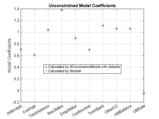
Figure contains an axes object. The axes object with title Unconstrained Model Coefficients, ylabel Model Coefficients contains 2 objects of type line. One or more of the lines displays its values using only markers These objects represent Calculated by fitConstrainedModel with defaults, Calculated by fimodel.

如表和绘图所示，模型系数匹配。您可以确信，fitConstrainedModel 的实现校准良好。

约束模型

在约束模型方法中，您要在线束下求解逻辑模型的系数 $b_{i}$ 值。支持的约束有边界、等式或不等式约束。系数要最大化为观测值 $i$ 定义的违约似然函数，如下所示：

$L_{i} = {p ({Default}_{i})}^{y_{i}} \times {(1 - p ({Default}_{i}))}^{1 - y_{i}}$

其中：

${p ({Default}_{i}) = \frac{1}{1 + e^{- b x_{i}}}}^{}$
$b = [b_{1} b_{2} . . . b_{K}]$ 是未知模型系数
$x_{i} = [x_{i1} x_{2} . . . x_{iK}]$ 是观测值 $i$ 处的预测值
$y_{i}$ 是响应值；值为 1 表示违约，值为 0 表示不违约

此公式适用于非加权数据。当观测值 i 的权重为 $w_{i}$ 时，这意味着有 $w_{i}$ 倍的观测值 i。因此，在观测值 i 时发生违约的概率是违约概率的乘积：

$p_{i} = \underset{w_{i} times}{{p ({Default}_{i})}^{y_{i}} * {p ({Default}_{i})}^{y_{i}} * . . . * {p ({Default}_{i})}^{y_{i}}} = {p ({Default}_{i})}^{{w_{i} * y}_{i}}$

同样，加权观测值 i 的不违约概率是：

${\hat{p}}_{i} = \underset{w_{i} times}{{p ({~ Default}_{i})}^{{1 - y}_{i}} * {p (~ {Default}_{i})}^{1 - y_{i}} * . . . * {p (~ {Default}_{i})}^{1 - y_{i}}} = {(1 - p ({Default}_{i}))}^{w_{i} * (1 - y_{i})}$

对于加权数据，如果权重为 $w_{i}$ 的给定观测值 i 存在违约，则就好像存在 $w_{i}$ 个该观测值，并且所有观测值或是全部违约，或是全部不违约。 $w_{i}$ 可能是整数，也可能非整数。

因此，对于加权数据，第一个方程中观测值 i 的违约似然函数变成

$L_{i} = {p ({Default}_{i})}^{{w_{i} * y}_{i}} \times {(1 - p ({Default}_{i}))}^{w_{i} * (1 - y_{i})}$

根据假设，所有违约都是独立事件，因此目标函数为

$L = L_{1} \times L_{2} \times . . . \times L_{N}$

或者，可用以下更方便的对数项表示：

$\log (L) = \sum_{i = 1}^{N} w_{i} * [y_{i} \log (p ({Default}_{i})) + (1 - y_{i}) \log (1 - p ({Default}_{i}))]$

对系数应用约束

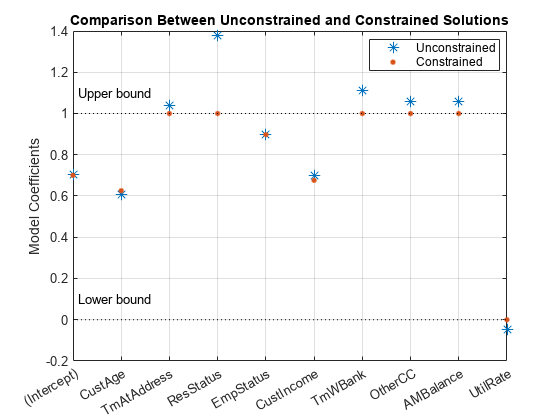
按照“使用 fitConstrainedModel 的无约束模型”部分所述校准无约束模型后，您可以求解受约束的模型系数。除了截距外，您可以选择下界和上界以使得 $0 \leq b_{i} \leq 1, \forall i = 1 . . . K$ 。此外，由于客户年龄和客户收入有些相关性，您还可以对它们的系数使用其他约束，例如， $| b_{C u s A g e} - b_{C u s t I n c o m e} | < 0.1$ 。本例中，预测变量 'CustAge' 和 'CustIncome' 的系数分别是 $b_{2}$ 和 $b_{6}$ 。

K  = length(sc.PredictorVars);
lb = [-Inf;zeros(K,1)];
ub = [Inf;ones(K,1)];
AIneq = [0 -1 0 0 0 1 0 0 0 0;0 -1 0 0 0 -1 0 0 0 0];
bIneq = [0.05;0.05];
Options = optimoptions('fmincon','SpecifyObjectiveGradient',true,'Display','off');
[sc3,mdl] = fitConstrainedModel(sc,'AInequality',AIneq,'bInequality',bIneq,...
    'LowerBound',lb,'UpperBound',ub,'Options',Options);

figure
plot(coeff1,'*','MarkerSize',8)
hold on
plot(mdl.Coefficients.Estimate,'.','MarkerSize',12)
line(xlim,[0 0],'color','k','linestyle',':')
line(xlim,[1 1],'color','k','linestyle',':')
text(1.1,0.1,'Lower bound')
text(1.1,1.1,'Upper bound')
grid on

xticklabels(mdl.Coefficients.Properties.RowNames)
ylabel('Model Coefficients')
title('Comparison Between Unconstrained and Constrained Solutions')
legend({'Unconstrained','Constrained'},'Location','best')

Figure contains an axes object. The axes object with title Comparison Between Unconstrained and Constrained Solutions, ylabel Model Coefficients contains 6 objects of type line, text. One or more of the lines displays its values using only markers These objects represent Unconstrained, Constrained.

显著性自助法

对于无约束问题，可使用标准公式计算 p 值，以评估哪些系数是显著的，而哪些系数将被拒绝。然而，对于约束问题，没有标准公式，显著性分析公式的推导也很复杂。一种实用的替代方法是通过自助法执行显著性分析。

在自助法中，当使用 fitConstrainedModel 时，将名称-值参量 'Bootstrap' 设置为 true，并为名称-值参量选择一个值 'BootstrapIter'。使用自助法意味着从原始观测值中选择 $NIter$ 个样本（有放回）。在每次迭代中，fitConstrainedModel 求解与“约束模型”部分相同的约束问题。fitConstrainedModel 获得每个系数 $b_{i}$ 的几个值（解），您可以将其绘制为 boxplot 或 histogram。使用箱线图或直方图，您可以检查中位数以评估系数是否偏离零以及系数偏离其均值的程度。

lb = [-Inf;zeros(K,1)];
ub = [Inf;ones(K,1)];
AIneq = [0 -1 0 0 0 1 0 0 0 0;0 1 0 0 0 -1 0 0 0 0];
bIneq = [0.05;0.05];
c0 = zeros(K,1);
NIter = 100;
Options = optimoptions('fmincon','SpecifyObjectiveGradient',true,'Display','off');
rng('default')

[sc,mdl] = fitConstrainedModel(sc,'AInequality',AIneq,'bInequality',bIneq,...
    'LowerBound',lb,'UpperBound',ub,'Bootstrap',true,'BootstrapIter',NIter,'Options',Options);

figure
boxplot(mdl.Bootstrap.Matrix,mdl.Coefficients.Properties.RowNames)
hold on
line(xlim,[0 0],'color','k','linestyle',':')
line(xlim,[1 1],'color','k','linestyle',':')
title('Bootstrapping with N = 100 Iterations')
ylabel('Model Coefficients')

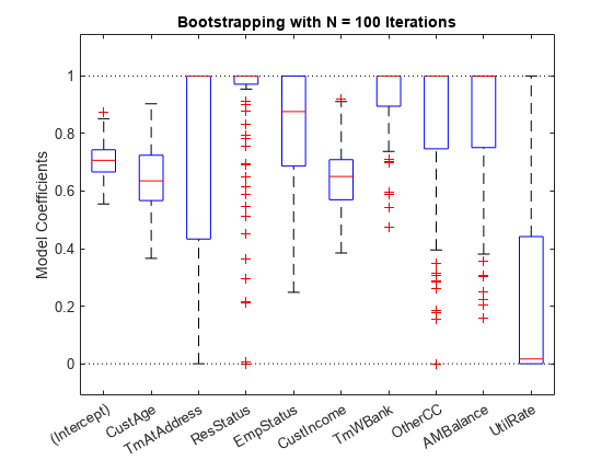
Figure contains an axes object. The axes object with title Bootstrapping with N = 100 Iterations, ylabel Model Coefficients contains 72 objects of type line. One or more of the lines displays its values using only markers

箱形图中的红实线表示中位数，底部和顶部边缘适用于 $25^{th}$ 和 $75^{th}$ 百分位数。“须线”是最小值和最大值，不包括离群值。虚线表示系数的下界和上界约束。在此示例中，系数不能为负。

为了帮助决定将在模型中保留哪些预测变量，需要评估每个系数为零的次数的比例。

Tol = 1e-6;
figure
bar(100*sum(mdl.Bootstrap.Matrix<= Tol)/NIter)
ylabel('% of Zeros')
title('Percentage of Zeros Over Bootstrap Iterations')
xticklabels(mdl.Coefficients.Properties.RowNames)
grid on

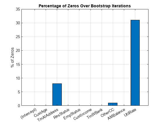
Figure contains an axes object. The axes object with title Percentage of Zeros Over Bootstrap Iterations, ylabel % of Zeros contains an object of type bar.

根据绘图，您可以拒绝 'UtilRate'，因为它具有最多数量的零值。您也可以决定拒绝 'TmAtAddress'，因为它显示为峰值，尽管该峰值较小。

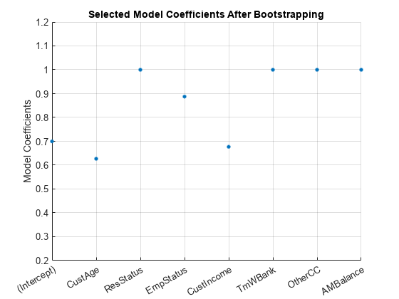
将相应的系数设置为零

要将相应的系数设置为零，需要将其上界设置为零，然后使用原始数据集重新求解模型。

ub(3) = 0;
ub(end) = 0;
[sc,mdl] = fitConstrainedModel(sc,'AInequality',AIneq,'bInequality',bIneq,'LowerBound',lb,'UpperBound',ub,'Options',Options);
Ind = (abs(mdl.Coefficients.Estimate) <= Tol);
ModelCoeff = mdl.Coefficients.Estimate(~Ind);
ModelPreds = mdl.Coefficients.Properties.RowNames(~Ind)';

figure
hold on
plot(ModelCoeff,'.','MarkerSize',12)
ylim([0.2 1.2])
ylabel('Model Coefficients')
xticklabels(ModelPreds)
title('Selected Model Coefficients After Bootstrapping')
grid on

Figure contains an axes object. The axes object with title Selected Model Coefficients After Bootstrapping, ylabel Model Coefficients contains a line object which displays its values using only markers.

将约束系数重新设置为 `creditscorecard`

现在您已经求解了约束系数，请使用 setmodel 设置模型的系数和预测变量。然后您可以计算（未缩放的）点数。

ModelPreds = ModelPreds(2:end);
sc = setmodel(sc,ModelPreds,ModelCoeff);
p = displaypoints(sc);

disp(p)

      Predictors               Bin              Points  
    ______________    _____________________    _________

    {'CustAge'   }    {'[-Inf,33)'        }     -0.16725
    {'CustAge'   }    {'[33,37)'          }     -0.14811
    {'CustAge'   }    {'[37,40)'          }    -0.065607
    {'CustAge'   }    {'[40,46)'          }     0.044404
    {'CustAge'   }    {'[46,48)'          }      0.21761
    {'CustAge'   }    {'[48,58)'          }      0.23404
    {'CustAge'   }    {'[58,Inf]'         }      0.49029
    {'CustAge'   }    {'<missing>'        }          NaN
    {'ResStatus' }    {'Tenant'           }    0.0044307
    {'ResStatus' }    {'Home Owner'       }      0.11932
    {'ResStatus' }    {'Other'            }      0.30048
    {'ResStatus' }    {'<missing>'        }          NaN
    {'EmpStatus' }    {'Unknown'          }    -0.077028
    {'EmpStatus' }    {'Employed'         }      0.31459
    {'EmpStatus' }    {'<missing>'        }          NaN
    {'CustIncome'}    {'[-Inf,29000)'     }     -0.43795
    {'CustIncome'}    {'[29000,33000)'    }    -0.097814
    {'CustIncome'}    {'[33000,35000)'    }     0.053667
    {'CustIncome'}    {'[35000,40000)'    }     0.081921
    {'CustIncome'}    {'[40000,42000)'    }     0.092364
    {'CustIncome'}    {'[42000,47000)'    }      0.23932
    {'CustIncome'}    {'[47000,Inf]'      }      0.42477
    {'CustIncome'}    {'<missing>'        }          NaN
    {'TmWBank'   }    {'[-Inf,12)'        }     -0.15547
    {'TmWBank'   }    {'[12,23)'          }    -0.031077
    {'TmWBank'   }    {'[23,45)'          }    -0.021091
    {'TmWBank'   }    {'[45,71)'          }      0.36703
    {'TmWBank'   }    {'[71,Inf]'         }      0.86888
    {'TmWBank'   }    {'<missing>'        }          NaN
    {'OtherCC'   }    {'No'               }     -0.16832
    {'OtherCC'   }    {'Yes'              }      0.15336
    {'OtherCC'   }    {'<missing>'        }          NaN
    {'AMBalance' }    {'[-Inf,558.88)'    }      0.34418
    {'AMBalance' }    {'[558.88,1254.28)' }    -0.012745
    {'AMBalance' }    {'[1254.28,1597.44)'}    -0.057879
    {'AMBalance' }    {'[1597.44,Inf]'    }     -0.19896
    {'AMBalance' }    {'<missing>'        }          NaN

使用未缩放的点数，您可以按照 Credit Scorecard Modeling Workflow 中其余部分的内容来计算分数和违约概率，并验证模型。

另请参阅

主题

外部网站

MATLAB 信用风险建模（53 分 10 秒）