fitConstrainedModel

Fit logistic regression model to Weight of Evidence (WOE) data subject to constraints on model coefficients

Syntax

[sc,mdl] = fitConstrainedModel(sc)

[sc,mdl]
= fitConstrainedModel(___,Name,Value)

Description

[sc,mdl] = fitConstrainedModel(sc) fits a logistic regression model to the Weight of Evidence (WOE) data subject to equality, inequality, or bound constraints on the model coefficients. fitConstrainedModel stores the model predictor names and corresponding coefficients in an updated creditscorecard object sc and returns the GeneralizedLinearModel object mdl which contains the fitted model.

example

[sc,mdl] = fitConstrainedModel(___,Name,Value) specifies options using one or more name-value pair arguments in addition to the input arguments in the previous syntax.

example

Examples

collapse all

Credit Scorecards with Constrained Logistic Regression Coefficients

Open Live Script

To compute scores for a creditscorecard object with constraints for equality, inequality, or bounds on the coefficients of the logistic regression model, use fitConstrainedModel. Unlike fitmodel, fitConstrainedModel solves for both the unconstrained and constrained problem. The current solver used to minimize an objective function for fitConstrainedModel is fmincon, from the Optimization Toolbox™.

This example has three main sections. First, fitConstrainedModel is used to solve for the coefficients in the unconstrained model. Then, fitConstrainedModel demonstrates how to use several types of constraints. Finally, fitConstrainedModel uses bootstrapping for the significance analysis to determine which predictors to reject from the model.

Create the creditscorecard Object and Bin data

load CreditCardData.mat
sc = creditscorecard(data,'IDVar','CustID');
sc = autobinning(sc);

Unconstrained Model Using fitConstrainedModel

Solve for the unconstrained coefficients using fitConstrainedModel with default values for the input parameters. fitConstrainedModel uses the internal optimization solver fmincon from the Optimization Toolbox™. If you do not set any constraints, fmincon treats the model as an unconstrained optimization problem. The default parameters for the LowerBound and UpperBound are -Inf and +Inf, respectively. For the equality and inequality constraints, the default is an empty numeric array.

[sc1,mdl1] = fitConstrainedModel(sc);
coeff1 = mdl1.Coefficients.Estimate;
disp(mdl1.Coefficients);

                   Estimate 
                   _________

    (Intercept)      0.70246
    CustAge           0.6057
    TmAtAddress       1.0381
    ResStatus         1.3794
    EmpStatus        0.89648
    CustIncome       0.70179
    TmWBank           1.1132
    OtherCC           1.0598
    AMBalance         1.0572
    UtilRate       -0.047597

Unlike fitmodel which gives p-values, when using fitConstrainedModel, you must use bootstrapping to find out which predictors are rejected from the model, when subject to constraints. This is illustrated in the "Significance Bootstrapping" section.

Using fitmodel to Compare the Results and Calibrate the Model

fitmodel fits a logistic regression model to the Weight-of-Evidence (WOE) data and there are no constraints. You can compare the results from the "Unconstrained Model Using fitConstrainedModel" section with those of fitmodel to verify that the model is well calibrated.

Now, solve the unconstrained problem by using fitmodel. Note that fitmodel and fitConstrainedModel use different solvers. While fitConstrainedModel uses fmincon, fitmodel uses stepwiseglm by default. To include all predictors from the start, set the 'VariableSelection' name-value pair argument of fitmodel to 'fullmodel'.

[sc2,mdl2] = fitmodel(sc,'VariableSelection','fullmodel','Display','off');
coeff2 = mdl2.Coefficients.Estimate;
disp(mdl2.Coefficients);

                   Estimate        SE         tStat        pValue  
                   _________    ________    _________    __________

    (Intercept)      0.70246    0.064039       10.969    5.3719e-28
    CustAge           0.6057     0.24934       2.4292      0.015131
    TmAtAddress       1.0381     0.94042       1.1039       0.26963
    ResStatus         1.3794      0.6526       2.1137      0.034538
    EmpStatus        0.89648     0.29339       3.0556     0.0022458
    CustIncome       0.70179     0.21866       3.2095     0.0013295
    TmWBank           1.1132     0.23346       4.7683    1.8579e-06
    OtherCC           1.0598     0.53005       1.9994      0.045568
    AMBalance         1.0572     0.36601       2.8884     0.0038718
    UtilRate       -0.047597     0.61133    -0.077858       0.93794

figure
plot(coeff1,'*')
hold on
plot(coeff2,'s')
xticklabels(mdl1.Coefficients.Properties.RowNames)
ylabel('Model Coefficients')
title('Unconstrained Model Coefficients')
legend({'Calculated by fitConstrainedModel with defaults','Calculated by fimodel'},'Location','best')
grid on

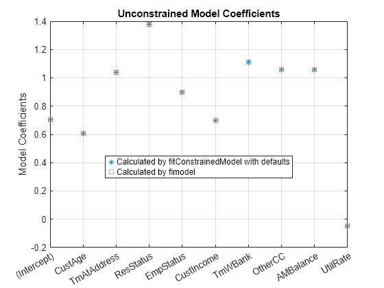
Figure contains an axes object. The axes object with title Unconstrained Model Coefficients, ylabel Model Coefficients contains 2 objects of type line. One or more of the lines displays its values using only markers These objects represent Calculated by fitConstrainedModel with defaults, Calculated by fimodel.

As both the tables and the plot show, the model coefficients match. You can be confident that this implementation of fitConstrainedModel is well calibrated.

Constrained Model

In the constrained model approach, you solve for the values of the coefficients $b_{i}$ of the logistic model, subject to constraints. The supported constraints are bound, equality, or inequality. The coefficients maximize the likelihood-of-default function defined, for observation $i$ , as:

$L_{i} = {p ({Default}_{i})}^{y_{i}} \times {(1 - p ({Default}_{i}))}^{1 - y_{i}}$

where:

${p ({Default}_{i}) = \frac{1}{1 + e^{- b x_{i}}}}^{}$
$b = [b_{1} b_{2} . . . b_{K}]$ is an unknown model coefficient
$x_{i} = [x_{i1} x_{2} . . . x_{iK}]$ is the predictor values at observation $i$
$y_{i}$ is the response value; a value of 1 represents default and a value of 0 represents non-default

This formula is for non-weighted data. When observation i has weight $w_{i}$ , it means that there are $w_{i}$ as many observations i. Therefore, the probability that default occurs at observation i is the product of the probabilities of default:

$p_{i} = \underset{w_{i} times}{{p ({Default}_{i})}^{y_{i}} * {p ({Default}_{i})}^{y_{i}} * . . . * {p ({Default}_{i})}^{y_{i}}} = {p ({Default}_{i})}^{{w_{i} * y}_{i}}$

Likewise, the probability of non-default for weighted observation i is:

${\hat{p}}_{i} = \underset{w_{i} times}{{p ({~ Default}_{i})}^{{1 - y}_{i}} * {p (~ {Default}_{i})}^{1 - y_{i}} * . . . * {p (~ {Default}_{i})}^{1 - y_{i}}} = {(1 - p ({Default}_{i}))}^{w_{i} * (1 - y_{i})}$

For weighted data, if there is default at a given observation i whose weight is $w_{i}$ , it is as if there was a $w_{i}$ count of that one observation, and all of them either all default, or all non-default. $w_{i}$ may or may not be an integer.

Therefore, for the weighted data, the likelihood-of-default function for observation i in the first equation becomes

$L_{i} = {p ({Default}_{i})}^{{w_{i} * y}_{i}} \times {(1 - p ({Default}_{i}))}^{w_{i} * (1 - y_{i})}$

By assumption, all defaults are independent events, so the objective function is

$L = L_{1} \times L_{2} \times . . . \times L_{N}$

or, in more convenient logarithmic terms:

$\log (L) = \sum_{i = 1}^{N} w_{i} * [y_{i} \log (p ({Default}_{i})) + (1 - y_{i}) \log (1 - p ({Default}_{i}))]$

Apply Constraints on the Coefficients

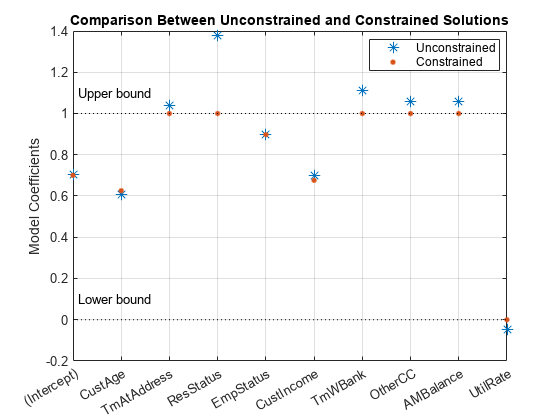
After calibrating the unconstrained model as described in the "Unconstrained Model Using fitConstrainedModel" section, you can solve for the model coefficients subject to constraints. You can choose lower and upper bounds such that $0 \leq b_{i} \leq 1, \forall i = 1 . . . K$ , except for the intercept. Also, since the customer age and customer income are somewhat correlated, you can also use additional constraints on their coefficients, for example, $| b_{C u s A g e} - b_{C u s t I n c o m e} | < 0.1$ . The coefficients corresponding to the predictors 'CustAge' and 'CustIncome' in this example are $b_{2}$ and $b_{6}$ , respectively.

K  = length(sc.PredictorVars);
lb = [-Inf;zeros(K,1)];
ub = [Inf;ones(K,1)];
AIneq = [0 -1 0 0 0 1 0 0 0 0;0 -1 0 0 0 -1 0 0 0 0];
bIneq = [0.05;0.05];
Options = optimoptions('fmincon','SpecifyObjectiveGradient',true,'Display','off');
[sc3,mdl] = fitConstrainedModel(sc,'AInequality',AIneq,'bInequality',bIneq,...
    'LowerBound',lb,'UpperBound',ub,'Options',Options);

figure
plot(coeff1,'*','MarkerSize',8)
hold on
plot(mdl.Coefficients.Estimate,'.','MarkerSize',12)
line(xlim,[0 0],'color','k','linestyle',':')
line(xlim,[1 1],'color','k','linestyle',':')
text(1.1,0.1,'Lower bound')
text(1.1,1.1,'Upper bound')
grid on

xticklabels(mdl.Coefficients.Properties.RowNames)
ylabel('Model Coefficients')
title('Comparison Between Unconstrained and Constrained Solutions')
legend({'Unconstrained','Constrained'},'Location','best')

Figure contains an axes object. The axes object with title Comparison Between Unconstrained and Constrained Solutions, ylabel Model Coefficients contains 6 objects of type line, text. One or more of the lines displays its values using only markers These objects represent Unconstrained, Constrained.

Significance Bootstrapping

For the unconstrained problem, standard formulas are available for computing p-values, which you use to evaluate which coefficients are significant and which are to be rejected. However, for the constrained problem, standard formulas are not available, and the derivation of formulas for significance analysis is complicated. A practical alternative is to perform significance analysis through bootstrapping.

In the bootstrapping approach, when using fitConstrainedModel, you set the name-value argument 'Bootstrap' to true and chose a value for the name-value argument 'BootstrapIter'. Bootstrapping means that $NIter$ samples (with replacement) from the original observations are selected. In each iteration, fitConstrainedModel solves for the same constrained problem as the "Constrained Model" section. fitConstrainedModel obtains several values (solutions) for each coefficient $b_{i}$ and you can plot these as a boxplot or histogram. Using the boxplot or histogram, you can examine the median values to evaluate whether the coefficients are away from zero and how much the coefficients deviate from their means.

lb = [-Inf;zeros(K,1)];
ub = [Inf;ones(K,1)];
AIneq = [0 -1 0 0 0 1 0 0 0 0;0 1 0 0 0 -1 0 0 0 0];
bIneq = [0.05;0.05];
c0 = zeros(K,1);
NIter = 100;
Options = optimoptions('fmincon','SpecifyObjectiveGradient',true,'Display','off');
rng('default')

[sc,mdl] = fitConstrainedModel(sc,'AInequality',AIneq,'bInequality',bIneq,...
    'LowerBound',lb,'UpperBound',ub,'Bootstrap',true,'BootstrapIter',NIter,'Options',Options);

figure
boxplot(mdl.Bootstrap.Matrix,mdl.Coefficients.Properties.RowNames)
hold on
line(xlim,[0 0],'color','k','linestyle',':')
line(xlim,[1 1],'color','k','linestyle',':')
title('Bootstrapping with N = 100 Iterations')
ylabel('Model Coefficients')

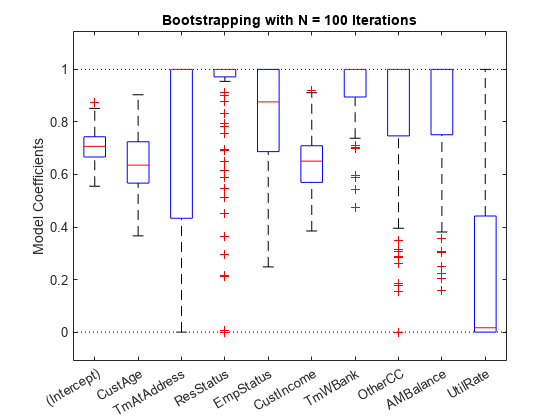
Figure contains an axes object. The axes object with title Bootstrapping with N = 100 Iterations, ylabel Model Coefficients contains 72 objects of type line. One or more of the lines displays its values using only markers

The solid red lines in the boxplot indicate that the median values and the bottom and top edges are for the $25^{th}$ and $75^{th}$ percentiles. The "whiskers" are the minimum and maximum values, not including outliers. The dotted lines represent the lower and upper bound constraints on the coefficients. In this example, the coefficients cannot be negative, by construction.

To help decide which predictors to keep in the model, assess the proportion of times each coefficient is zero.

Tol = 1e-6;
figure
bar(100*sum(mdl.Bootstrap.Matrix<= Tol)/NIter)
ylabel('% of Zeros')
title('Percentage of Zeros Over Bootstrap Iterations')
xticklabels(mdl.Coefficients.Properties.RowNames)
grid on

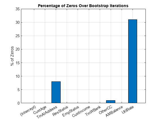
Figure contains an axes object. The axes object with title Percentage of Zeros Over Bootstrap Iterations, ylabel % of Zeros contains an object of type bar.

Based on the plot, you can reject 'UtilRate' since it has the highest number of zero values. You can also decide to reject 'TmAtAddress' since it shows a peak, albeit small.

Set the Corresponding Coefficients to Zero

To set the corresponding coefficients to zero, set their upper bound to zero and solve the model again using the original data set.

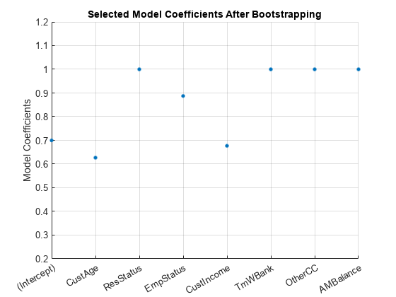
ub(3) = 0;
ub(end) = 0;
[sc,mdl] = fitConstrainedModel(sc,'AInequality',AIneq,'bInequality',bIneq,'LowerBound',lb,'UpperBound',ub,'Options',Options);
Ind = (abs(mdl.Coefficients.Estimate) <= Tol);
ModelCoeff = mdl.Coefficients.Estimate(~Ind);
ModelPreds = mdl.Coefficients.Properties.RowNames(~Ind)';

figure
hold on
plot(ModelCoeff,'.','MarkerSize',12)
ylim([0.2 1.2])
ylabel('Model Coefficients')
xticklabels(ModelPreds)
title('Selected Model Coefficients After Bootstrapping')
grid on

Figure contains an axes object. The axes object with title Selected Model Coefficients After Bootstrapping, ylabel Model Coefficients contains a line object which displays its values using only markers.

Set Constrained Coefficients Back Into the creditscorecard

Now that you have solved for the constrained coefficients, use setmodel to set the model's coefficients and predictors. Then you can compute the (unscaled) points.

ModelPreds = ModelPreds(2:end);
sc = setmodel(sc,ModelPreds,ModelCoeff);
p = displaypoints(sc);

disp(p)

      Predictors               Bin              Points  
    ______________    _____________________    _________

    {'CustAge'   }    {'[-Inf,33)'        }     -0.16725
    {'CustAge'   }    {'[33,37)'          }     -0.14811
    {'CustAge'   }    {'[37,40)'          }    -0.065607
    {'CustAge'   }    {'[40,46)'          }     0.044404
    {'CustAge'   }    {'[46,48)'          }      0.21761
    {'CustAge'   }    {'[48,58)'          }      0.23404
    {'CustAge'   }    {'[58,Inf]'         }      0.49029
    {'CustAge'   }    {'<missing>'        }          NaN
    {'ResStatus' }    {'Tenant'           }    0.0044307
    {'ResStatus' }    {'Home Owner'       }      0.11932
    {'ResStatus' }    {'Other'            }      0.30048
    {'ResStatus' }    {'<missing>'        }          NaN
    {'EmpStatus' }    {'Unknown'          }    -0.077028
    {'EmpStatus' }    {'Employed'         }      0.31459
    {'EmpStatus' }    {'<missing>'        }          NaN
    {'CustIncome'}    {'[-Inf,29000)'     }     -0.43795
    {'CustIncome'}    {'[29000,33000)'    }    -0.097814
    {'CustIncome'}    {'[33000,35000)'    }     0.053667
    {'CustIncome'}    {'[35000,40000)'    }     0.081921
    {'CustIncome'}    {'[40000,42000)'    }     0.092364
    {'CustIncome'}    {'[42000,47000)'    }      0.23932
    {'CustIncome'}    {'[47000,Inf]'      }      0.42477
    {'CustIncome'}    {'<missing>'        }          NaN
    {'TmWBank'   }    {'[-Inf,12)'        }     -0.15547
    {'TmWBank'   }    {'[12,23)'          }    -0.031077
    {'TmWBank'   }    {'[23,45)'          }    -0.021091
    {'TmWBank'   }    {'[45,71)'          }      0.36703
    {'TmWBank'   }    {'[71,Inf]'         }      0.86888
    {'TmWBank'   }    {'<missing>'        }          NaN
    {'OtherCC'   }    {'No'               }     -0.16832
    {'OtherCC'   }    {'Yes'              }      0.15336
    {'OtherCC'   }    {'<missing>'        }          NaN
    {'AMBalance' }    {'[-Inf,558.88)'    }      0.34418
    {'AMBalance' }    {'[558.88,1254.28)' }    -0.012745
    {'AMBalance' }    {'[1254.28,1597.44)'}    -0.057879
    {'AMBalance' }    {'[1597.44,Inf]'    }     -0.19896
    {'AMBalance' }    {'<missing>'        }          NaN

Using the unscaled points, you can follow the remainder of the Credit Scorecard Modeling Workflow to compute scores and probabilities of default and to validate the model.

Input Arguments

collapse all

`sc` — Credit scorecard model
`creditscorecard` object

Credit scorecard model, specified as a creditscorecard object. Use creditscorecard to create a creditscorecard object.

Name-Value Arguments

Specify optional pairs of arguments as Name1=Value1,...,NameN=ValueN, where Name is the argument name and Value is the corresponding value. Name-value arguments must appear after other arguments, but the order of the pairs does not matter.

Before R2021a, use commas to separate each name and value, and enclose Name in quotes.

Example: [sc,mdl] = fitConstrainedModel(sc,'LowerBound',2,'UpperBound',100)

`PredictorVars` — Predictor variables for fitting `creditscorecard` object
all predictors in the `creditscorecard` object (default) | cell array of character vectors

Predictor variables for fitting the creditscorecard object, specified as the comma-separated pair consisting of 'PredictorVars' and a cell array of character vectors. If you provide predictor variables, then the function updates the creditscorecard object property PredictorsVars. The order of predictors in the original dataset is enforced, regardless of the order in which 'PredictorVars' is provided. When not provided, the predictors used to create the creditscorecard object (by using creditscorecard) are used.

Data Types: cell

`LowerBound` — Lower bound
`-Inf` (default) | scalar | vector

Lower bound, specified as the comma-separated pair consisting of 'LowerBound' and a scalar or a real vector of length N+1, where N is the number of model coefficients in the creditscorecard object.

Data Types: double

`UpperBound` — Upper bound
`Inf` (default) | scalar | vector

Upper bound, specified as the comma-separated pair consisting of 'UpperBound' and a scalar or a real vector of length N+1, where N is the number of model coefficients in the creditscorecard object.

Data Types: double

`AInequality` — Matrix of linear inequality constraints
`[]` (default) | matrix

Matrix of linear inequality constraints, specified as the comma-separated pair consisting of 'AInequality' and a real M-by-N+1 matrix, where M is the number of constraints and N is the number of model coefficients in the creditscorecard object.

Data Types: double

`bInequality` — Vector of linear inequality constraints
`[]` (default) | vector

Vector of linear inequality constraints, specified as the comma-separated pair consisting of 'bInequality' and a real M-by-1 vector, where M is the number of constraints.

Data Types: double

`AEquality` — Matrix of linear equality constraints
`[]` (default) | matrix

Matrix of linear equality constraints, specified as the comma-separated pair consisting of 'AEquality' and a real M-by-N+1 matrix, where M is the number of constraints and N is the number of model coefficients in the creditscorecard object.

Data Types: double

`bEquality` — Vector of linear equality constraints
`[]` (default) | vector

Vector of linear equality constraints, specified as the comma-separated pair consisting of 'bEquality' and a real M-by-1 vector, where M is the number of constraints.

Data Types: double

`Bootstrap` — Indicator that bootstrapping defines the solution accuracy
`false` (default) | logical with a value of `true` or `false`

Indicator that bootstrapping defines the solution accuracy, specified as the comma-separated pair consisting of 'Bootstrap' and a logical with a value of true or false.

Data Types: logical

`BootstrapIter` — Number of bootstrapping iterations
`100` (default) | positive integer

Number of bootstrapping iterations, specified as the comma-separated pair consisting of 'BootstrapIter' and a positive integer.

Data Types: double

`Options` — `optimoptions` object
`optimoptions('fmincon','SpecifiedObjectiveGradient',true,'Display','off')` (default) | object

optimoptions object, specified as the comma-separated pair consisting of 'Options' and an optimoptions object. You can create the object by using optimoptions from Optimization Toolbox™.

Data Types: object

Output Arguments

collapse all

`sc` — Credit scorecard model
`creditscorecard` object

Credit scorecard model, returned as an updated creditscorecard object. The creditscorecard object contains information about the model predictors and coefficients that fit the WOE data. For more information on using the creditscorecard object, see creditscorecard.

`mdl` — Fitted logistic model
`GeneralizedLinearModel` object

Fitted logistic model, returned as a GeneralizedLinearModel object containing the fitted model. For more information on a GeneralizedLinearModel object, see GeneralizedLinearModel.

Note

If you specify the optional WeightsVar argument when creating a creditscorecard object, then mdl uses the weighted counts with stepwiseglm and fitglm.

The mdl structure has the following fields:

Coefficients is a table in which the RowNames property contains the names of the model coefficients and has a single column, 'Estimate', containing the solution.
Bootstrap exists when 'Bootstrap' is set to true, and has two fields:
- CI contains the 95% confidence interval for the solution.
- Matrix an NIter-by-N matrix of coefficients, where NIter is the number of bootstrap iterations and N is the number of model coefficients.
Solver has three fields:
- Options additional information on the algorithm and solution.
- ExitFlag contains an integer that codes the reason why the solver stopped. For more information, see fmincon.
- Output is a structure with additional information on the optimization process.

More About

collapse all

Model Coefficients

When you use fitConstrainedModel to solve for the model coefficients, the function solves for the same number of parameters as predictor variables you specify, plus one additional coefficient for the intercept.

The first coefficient corresponds to the intercept. If you provide predictor variables using the 'PredictorVars' optional input argument, then fitConstrainedModel updates the creditscorecard object property PredictorsVars. The order of predictors in the original dataset is enforced, regardless of the order in which 'PredictorVars' is provided. When not provided, the predictors used to create the creditscorecard object (by using creditscorecard) are used.

Calibration

The constrained model is first calibrated such that, when unconstrained, the solution is identical, within a certain tolerance, to the solution given by fitmodel, with the'fullmodel' choice for the name-value argument 'VariableSelection'.

As an exercise, you can test the calibration by leaving all name-value parameters of fitConstrainedModel to their default values. The solutions are identical to within a 10^-6 to 10^-5 tolerance.

Calibration with Weights and Missing Data

If the credit scorecard data contains observation weights, the fitConstrainedModel function uses the weights to calibrate the model coefficients.

For credit scorecard data with no missing data and no weights, the likelihood function for observation i is

$\begin{array}{l} L_{i} = p (^{{Default}_{i}) y_{i}} \times (^{1 - p ({Default}_{i})) 1 - y_{i}} \\ where p {(Default}_{i}) = \frac{1}{(1 + e^{- b x_{i}})} \end{array}$

where:

b = [b₁ b₂...b_K] is for unknown model coefficients
x_i = [x_i1 x_i2...x_iK] is the predictor values at observation i
y_i is the response value of 1 (the default) or a value of 0.

When observation i has weight w_i, it means that there are w_i observations. Because of the independence of defaults between observations, the probability that there is default at observation i is the product of the probabilities of default

$\begin{array}{l} p_{i} = p (^{{Default}_{i}) y_{i}} * p (^{{Default}_{i}) y_{i}} * ... * p (^{{Default}_{i}) y_{i}} = p (^{{Default}_{i}) w_{i} * y_{i}} \\ w_{i} times \end{array}$

Likewise, the probability of non-default for weighted observation i is

$\begin{array}{l} {\hat{p}}_{i} = p (^{~ {Default}_{i}) 1 - y_{i}} * p (^{~ {Default}_{i}) 1 - y_{i}} * ... * p (^{~ {Default}_{i}) 1 - y_{i}} = (1 - p (^{{Default}_{i}) w_{i} * (1 - y_{i})} \\ w_{i} times \end{array}$

For weighted data, if there is default at a given observation i whose weight is w_i, it is as if there was w_i defaults of that one observation, and all of them either all default, or all non-default. w_i may or may not be an integer. Therefore, the likelihood function for observation i becomes

$L_{i} = p {({Default}_{i})}^{w_{i} * y_{i}} \times {(1 - p ({Default}_{i}))}^{w_{i} * (1 - y_{i})}$

Likewise, for data with missing observations (NaN, <undefined>, or “Missing”), the model is calibrated by comparing the unconstrained case with results given by fitglm. Where the data contains missing observations, the WOE input matrix has NaN values. The NaN values do not pose any issue for fitglm (unconstrained), or fmincon (constrained). The only edge case is if all observations of a given predictor are missing, in which case, that predictor is discarded from the model.

Bootstrapping

Bootstrapping is a method for estimating the accuracy of the solution obtained after iterating the objective function NIter times.

When 'Bootstrap' is set to true, the fitConstrainedModel function performs sampling with replacement of the WOE values and is passed to the objective function. At the end of the iterative process, the solutions are stored in a NIter-by-N+1 matrix, where N is the number of model coefficients.

The 95% confidence interval (CI) returned in the output structure mdl.Bootstrap contains the values of the coefficients at the 25th and 97.5th percentiles.

Models

A logistic regression model is used in the creditscorecard object.

For the model, the probability of being “Bad” is given by ProbBad = exp(-s) / (1 + exp(-s)).

References

[1] Anderson, R. The Credit Scoring Toolkit. Oxford University Press, 2007.

[2] Refaat, M. Credit Risk Scorecards: Development and Implementation Using SAS. lulu.com, 2011.

Version History

Introduced in R2019a

fitConstrainedModel

Syntax

Description

Examples

Credit Scorecards with Constrained Logistic Regression Coefficients

Input Arguments

`sc` — Credit scorecard model
`creditscorecard` object

Name-Value Arguments

`PredictorVars` — Predictor variables for fitting `creditscorecard` object
all predictors in the `creditscorecard` object (default) | cell array of character vectors

`LowerBound` — Lower bound
`-Inf` (default) | scalar | vector

`UpperBound` — Upper bound
`Inf` (default) | scalar | vector

`AInequality` — Matrix of linear inequality constraints
`[]` (default) | matrix

`bInequality` — Vector of linear inequality constraints
`[]` (default) | vector

`AEquality` — Matrix of linear equality constraints
`[]` (default) | matrix

`bEquality` — Vector of linear equality constraints
`[]` (default) | vector

`Bootstrap` — Indicator that bootstrapping defines the solution accuracy
`false` (default) | logical with a value of `true` or `false`

`BootstrapIter` — Number of bootstrapping iterations
`100` (default) | positive integer

`Options` — `optimoptions` object
`optimoptions('fmincon','SpecifiedObjectiveGradient',true,'Display','off')` (default) | object

Output Arguments

`sc` — Credit scorecard model
`creditscorecard` object

`mdl` — Fitted logistic model
`GeneralizedLinearModel` object

More About

Model Coefficients

Calibration

Calibration with Weights and Missing Data

Bootstrapping

Models

References

Version History

See Also

Topics

fitConstrainedModel

Syntax

Description

Examples

Credit Scorecards with Constrained Logistic Regression Coefficients

Input Arguments

sc — Credit scorecard model creditscorecard object

Name-Value Arguments

PredictorVars — Predictor variables for fitting creditscorecard object all predictors in the creditscorecard object (default) | cell array of character vectors

LowerBound — Lower bound -Inf (default) | scalar | vector

UpperBound — Upper bound Inf (default) | scalar | vector

AInequality — Matrix of linear inequality constraints [] (default) | matrix

bInequality — Vector of linear inequality constraints [] (default) | vector

AEquality — Matrix of linear equality constraints [] (default) | matrix

bEquality — Vector of linear equality constraints [] (default) | vector

Bootstrap — Indicator that bootstrapping defines the solution accuracy false (default) | logical with a value of true or false

BootstrapIter — Number of bootstrapping iterations 100 (default) | positive integer

Options — optimoptions object optimoptions('fmincon','SpecifiedObjectiveGradient',true,'Display','off') (default) | object

Output Arguments

sc — Credit scorecard model creditscorecard object

mdl — Fitted logistic model GeneralizedLinearModel object

More About

Model Coefficients

Calibration

Calibration with Weights and Missing Data

Bootstrapping

Models

References

Version History

See Also

Topics

`sc` — Credit scorecard model
`creditscorecard` object

`PredictorVars` — Predictor variables for fitting `creditscorecard` object
all predictors in the `creditscorecard` object (default) | cell array of character vectors

`LowerBound` — Lower bound
`-Inf` (default) | scalar | vector

`UpperBound` — Upper bound
`Inf` (default) | scalar | vector

`AInequality` — Matrix of linear inequality constraints
`[]` (default) | matrix

`bInequality` — Vector of linear inequality constraints
`[]` (default) | vector

`AEquality` — Matrix of linear equality constraints
`[]` (default) | matrix

`bEquality` — Vector of linear equality constraints
`[]` (default) | vector

`Bootstrap` — Indicator that bootstrapping defines the solution accuracy
`false` (default) | logical with a value of `true` or `false`

`BootstrapIter` — Number of bootstrapping iterations
`100` (default) | positive integer

`Options` — `optimoptions` object
`optimoptions('fmincon','SpecifiedObjectiveGradient',true,'Display','off')` (default) | object

`sc` — Credit scorecard model
`creditscorecard` object

`mdl` — Fitted logistic model
`GeneralizedLinearModel` object