使用 `ga` 的约束最小化，基于问题

此示例说明如何使用基于问题的方法中的 ga 来最小化受非线性不等式约束和边界的目标函数。有关该问题基于求解器的版本，请参阅使用遗传算法进行约束最小化。

约束最小化问题

对于这个问题，最小化的适应度函数是二维变量 X 和 Y 的简单函数。

camxy = @(X,Y)(4 - 2.1.*X.^2 + X.^4./3).*X.^2 + X.*Y + (-4 + 4.*Y.^2).*Y.^2;

该函数在 Dixon 和 Szego [1] 中有描述。

此外，该问题具有非线性约束和边界。

   x*y + x - y + 1.5 <= 0  (nonlinear constraint)
   10 - x*y <= 0           (nonlinear constraint)
   0 <= x <= 1             (bound)
   0 <= y <= 13            (bound)

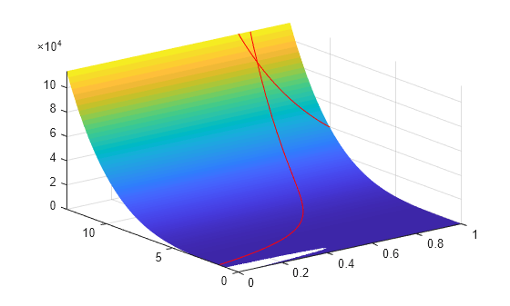
在适应度函数的曲面图上绘制非线性约束区域。这些约束将解决解限制在两条红色曲线上方的小区域内。

x1 = linspace(0,1);
y1 = (-x1 - 1.5)./(x1 - 1);
y2 = 10./x1;
[X,Y] = meshgrid(x1,linspace(0,13));
Z = camxy(X,Y);
surf(X,Y,Z,"LineStyle","none")
hold on
z1 = camxy(x1,y1);
z2 = camxy(x1,y2);
plot3(x1,y1,z1,'r-',x1,y2,z2,'r-')
xlim([0 1])
ylim([0 13])
zlim([0,max(Z,[],"all")])
hold off

Figure contains an axes object. The axes object contains 3 objects of type surface, line.

创建优化变量、问题和约束

为了设置这个问题，创建优化变量 x 和 y。创建变量时设置边界。

x = optimvar("x","LowerBound",0,"UpperBound",1);
y = optimvar("y","LowerBound",0,"UpperBound",13);

将目标创建为优化表达式。

cam = camxy(x,y);

用这个目标函数创建一个优化问题。

prob = optimproblem("Objective",cam);

创建两个非线性不等式约束，并将它们包含在问题中。

prob.Constraints.cons1 = x*y + x - y + 1.5 <= 0;
prob.Constraints.cons2 = 10 - x*y <= 0;

检查此问题。

show(prob)

  OptimizationProblem : 

	Solve for:
       x, y

	minimize :
       (((((4 - (2.1 .* x.^2)) + (x.^4 ./ 3)) .* x.^2) + (x .* y)) + (((-4) + (4 .* y.^2)) .* y.^2))


	subject to cons1:
       ((((x .* y) + x) - y) + 1.5) <= 0

	subject to cons2:
       (10 - (x .* y)) <= 0

	variable bounds:
       0 <= x <= 1

       0 <= y <= 13

求解问题

求解问题，指定 ga 求解器。

[sol,fval] = solve(prob,"Solver","ga")

Solving problem using ga.
Optimization finished: average change in the fitness value less than options.FunctionTolerance and constraint violation is less than options.ConstraintTolerance.

sol = struct with fields:
    x: 0.8122
    y: 12.3103

fval = 
9.1268e+04

添加可视化

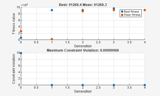
要观察求解器的进度，请指定选择两个绘图函数的选项。绘图函数 gaplotbestf 绘制每次迭代中的最佳目标函数值，绘图函数 gaplotmaxconstr 绘制每次迭代中的最大约束违反。在元胞数组中设置这两个绘图函数。另外，通过将 Display 选项设置为 'iter'，在命令窗口中显示有关求解器进度的信息。

options = optimoptions(@ga,...
    'PlotFcn',{@gaplotbestf,@gaplotmaxconstr},...
    'Display','iter');

运行求解器，包括 options 参量。

[sol,fval] = solve(prob,"Solver","ga","Options",options)

Solving problem using ga.

Single objective optimization:
2 Variables
2 Nonlinear inequality constraints

Options:
CreationFcn:       @gacreationuniform
CrossoverFcn:      @crossoverscattered
SelectionFcn:      @selectionstochunif
MutationFcn:       @mutationadaptfeasible

                              Best       Max        Stall
Generation  Func-count        f(x)     Constraint  Generations
    1           2520       91357.8            0      0
    2           4982       91324.1     4.55e-05      0
    3           7914       97166.6            0      0
    4          16145       91268.4    0.0009997      0
Optimization finished: average change in the fitness value less than options.FunctionTolerance and constraint violation is less than options.ConstraintTolerance.

Figure Genetic Algorithm contains 2 axes objects. Axes object 1 with title Best: 91268.4 Mean: 91268.3, xlabel Generation, ylabel Fitness value contains 2 objects of type scatter. These objects represent Best fitness, Mean fitness. Axes object 2 with title Maximum Constraint Violation: 0.000999679, xlabel Generation, ylabel Constraint violation contains an object of type scatter.

sol = struct with fields:
    x: 0.8123
    y: 12.3103

fval = 
9.1268e+04

非线性约束导致 ga 在每次迭代时解决许多子问题。从绘图和迭代显示可以看出，解过程只有几次迭代。但是，迭代显示中的 Func-count 列显示每次迭代有许多函数计算。

不支持的函数

如果您的目标或非线性约束函数不受支持（请参阅优化变量和表达式支持的运算），请使用 fcn2optimexpr 将它们转换为适合基于问题的方法的形式。例如，假设您有约束 $x y \geq 10$ 而不是约束 $I_{1} (x) + I_{1} (y) \geq 10$ ，其中 $I_{1} (x)$ 是修改后的贝塞尔函数 besseli(1,x)。（贝塞尔函数不是受支持的函数。）使用 fcn2optimexpr 创建此约束。首先，为 $I_{1} (x) + I_{1} (y)$ 创建一个优化表达式。

bfun = fcn2optimexpr(@(t,u)besseli(1,t) + besseli(1,u),x,y);

接下来，将约束 cons2 替换为约束 bfun >= 10。

prob.Constraints.cons2 = bfun >= 10;

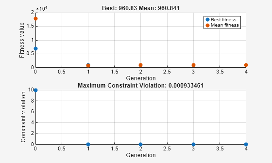
求解。由于约束区域不同，其解也不同。

[sol2,fval2] = solve(prob,"Solver","ga","Options",options)

Solving problem using ga.

Single objective optimization:
2 Variables
2 Nonlinear inequality constraints

Options:
CreationFcn:       @gacreationuniform
CrossoverFcn:      @crossoverscattered
SelectionFcn:      @selectionstochunif
MutationFcn:       @mutationadaptfeasible

                              Best       Max        Stall
Generation  Func-count        f(x)     Constraint  Generations
    1           2512       974.044            0      0
    2           4974       960.998            0      0
    3           7436        963.12            0      0
    4          12001        960.83    0.0009335      0
Optimization finished: average change in the fitness value less than options.FunctionTolerance and constraint violation is less than options.ConstraintTolerance.

Figure Genetic Algorithm contains 2 axes objects. Axes object 1 with title Best: 960.83 Mean: 960.841, xlabel Generation, ylabel Fitness value contains 2 objects of type scatter. These objects represent Best fitness, Mean fitness. Axes object 2 with title Maximum Constraint Violation: 0.000933461, xlabel Generation, ylabel Constraint violation contains an object of type scatter.

sol2 = struct with fields:
    x: 0.4999
    y: 3.9979

fval2 = 
960.8300

参考资料

[1] Dixon, L. C. W., and G .P. Szego (eds.).Towards Global Optimisation 2.North-Holland:Elsevier Science Ltd., Amsterdam, 1978.

另请参阅

ga | solve | fcn2optimexpr

使用 ga 的约束最小化，基于问题