Develop Camera Processing Pipeline Using Deep Learning
This example shows how to convert RAW camera data to an aesthetically pleasing color image using a U-Net.
DSLRs and many modern phone cameras offer the ability to save data collected directly from the camera sensor as a RAW file. Each pixel of RAW data corresponds directly to the amount of light captured by a corresponding camera photosensor. The data depends on fixed characteristics of the camera hardware, such as the sensitivity of each photosensor to a particular range of wavelengths of the electromagnetic spectrum. The data also depends on camera acquisition settings such as exposure time, and factors of the scene such as the light source.
Demosaicing is the only required operation to convert single-channel RAW data to a three-channel RGB image. However, without additional image processing operations, the resulting RGB image has subjectively poor visual quality.
A traditional image processing pipeline performs a combination of additional operations including denoising, linearization, white-balancing, color correction, brightness adjustment, and contrast adjustment [1]. The challenge of designing a pipeline lies in refining algorithms to optimize the subjective appearance of the final RGB image regardless of variations in the scene and acquisition settings.
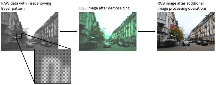
Deep learning techniques enable direct RAW to RGB conversion without the necessity of developing a traditional processing pipeline. For instance, one technique compensates for underexposure when converting RAW images to RGB [2]. This example shows how to convert RAW images from a lower end phone camera to RGB images that approximate the quality of a higher end DSLR camera.
Download Zurich RAW to RGB Data Set
This example uses the Zurich RAW to RGB data set [3]. The size of the data set is 22 GB. The data set contains 48,043 spatially registered pairs of RAW and RGB training image patches of size 448-by-448. The data set contains two separate test sets. One test set consists of 1,204 spatially registered pairs of RAW and RGB image patches of size 448-by-448. The other test set consists of unregistered full-resolution RAW and RGB images.
Specify dataDir as the desired location of the data.
dataDir = fullfile(tempdir,"ZurichRAWToRGB");To download the data set, go to https://data.vision.ee.ethz.ch/ihnatova/public/zr2d/Zurich-RAW-to-DSLR-Dataset.zip. Extract the data into the directory specified by the dataDir variable. When extracted successfully, dataDir contains three directories named full_resolution, test, and train.
Create Datastores for Training, Validation, and Testing
Create Datastore for RGB Image Patch Training Data
Create an imageDatastore that reads the target RGB training image patches acquired using a high-end Canon DSLR.
trainImageDir = fullfile(dataDir,"train");
dsTrainRGB = imageDatastore(fullfile(trainImageDir,"canon"),ReadSize=16);
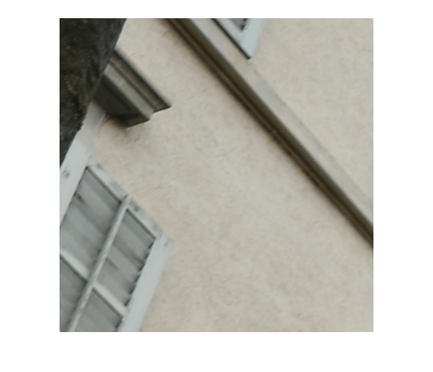
Preview an RGB training image patch.
groundTruthPatch = preview(dsTrainRGB);
imshow(groundTruthPatch)
Create Datastore for RAW Image Patch Training Data
Create an imageDatastore that reads the input RAW training image patches acquired using a Huawei phone camera. The RAW images are captured with 10-bit precision and are represented as both 8-bit and 16-bit PNG files. The 8-bit files provide a compact representation of patches with data in the range [0, 255]. No scaling has been done on any of the RAW data.
dsTrainRAW = imageDatastore(fullfile(trainImageDir,"huawei_raw"),ReadSize=16);Preview an input RAW training image patch. The datastore reads this patch as an 8-bit uint8 image because the sensor counts are in the range [0, 255]. To simulate the 10-bit dynamic range of the training data, divide the image intensity values by 4. If you zoom in on the image, then you can see the RGGB Bayer pattern.
inputPatch = preview(dsTrainRAW);
inputPatchRAW = inputPatch/4;
imshow(inputPatchRAW)

To simulate the minimal traditional processing pipeline, demosaic the RGGB Bayer pattern of the RAW data using the demosaic function. Display the processed image and brighten the display. Compared to the target RGB image, the minimally-processed RGB image is dark and has imbalanced colors and noticeable artifacts. A trained RAW-to-RGB network performs preprocessing operations so that the output RGB image resembles the target image.
inputPatchRGB = demosaic(inputPatch,"rggb");
imshow(rescale(inputPatchRGB))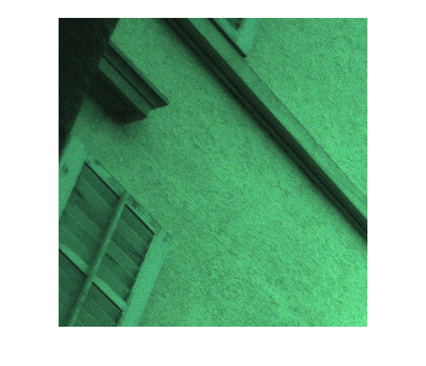
Partition Test Images into Validation and Test Sets
The test data contains RAW and RGB image patches and full-sized images. This example partitions the test image patches into a validation set and test set. The example uses the full-sized test images for qualitative testing only. See Evaluate Trained Image Processing Pipeline on Full-Sized Images.
Create image datastores that read the RAW and RGB test image patches.
testImageDir = fullfile(dataDir,"test");
dsTestRAW = imageDatastore(fullfile(testImageDir,"huawei_raw"),ReadSize=16);
dsTestRGB = imageDatastore(fullfile(testImageDir,"canon"),ReadSize=16);
Randomly split the test data into two sets for validation and training. The validation data set contains 200 images. The test set contains the remaining images.
numTestImages = dsTestRAW.numpartitions;
numValImages = 200;

testIdx = randperm(numTestImages);
validationIdx = testIdx(1:numValImages);
testIdx = testIdx(numValImages+1:numTestImages);

dsValRAW = subset(dsTestRAW,validationIdx);
dsValRGB = subset(dsTestRGB,validationIdx);

dsTestRAW = subset(dsTestRAW,testIdx);
dsTestRGB = subset(dsTestRGB,testIdx);
Preprocess and Augment Data
The sensor acquires color data in a repeating Bayer pattern that includes one red, two green, and one blue photosensor. Preprocess the data into a four-channel image expected of the network using the transform function. The transform function processes the data using the operations specified in the preprocessRAWDataForRAWToRGB helper function. The helper function is attached to the example as a supporting file.
The preprocessRAWDataForRAWToRGB helper function converts an H-by-W-by-1 RAW image to an H/2-by-W/2-by-4 multichannel image consisting of one red, two green, and one blue channel.

The function also casts the data to data type single scaled to the range [0, 1].
dsTrainRAW = transform(dsTrainRAW,@preprocessRAWDataForRAWToRGB);
dsValRAW = transform(dsValRAW,@preprocessRAWDataForRAWToRGB);
dsTestRAW = transform(dsTestRAW,@preprocessRAWDataForRAWToRGB);
The target RGB images are stored on disk as unsigned 8-bit data. To make the computation of metrics and the network design more convenient, preprocess the target RGB training images using the transform function and the preprocessRGBDataForRAWToRGB helper function. The helper function is attached to the example as a supporting file.
The preprocessRGBDataForRAWToRGB helper function casts images to data type single scaled to the range [0, 1].
dsTrainRGB = transform(dsTrainRGB,@preprocessRGBDataForRAWToRGB);
dsValRGB = transform(dsValRGB,@preprocessRGBDataForRAWToRGB);
Combine the input RAW and target RGB data for the training, validation, and test image sets by using the combine function.
dsTrain = combine(dsTrainRAW,dsTrainRGB);
dsVal = combine(dsValRAW,dsValRGB);
dsTest = combine(dsTestRAW,dsTestRGB);
Randomly augment the training data using the transform function and the augmentDataForRAWToRGB helper function. The helper function is attached to the example as a supporting file.
The augmentDataForRAWToRGB helper function randomly applies 90 degree rotation and horizontal reflection to pairs of input RAW and target RGB training images.
dsTrainAug = transform(dsTrain,@augmentDataForRAWToRGB);
Preview the augmented training data.
exampleAug = preview(dsTrainAug)
exampleAug=8×2 cell array
    224×224×4 single    448×448×3 single
    224×224×4 single    448×448×3 single
    224×224×4 single    448×448×3 single
    224×224×4 single    448×448×3 single
    224×224×4 single    448×448×3 single
    224×224×4 single    448×448×3 single
    224×224×4 single    448×448×3 single
    224×224×4 single    448×448×3 single
Display the network input and target image in a montage. The network input has four channels, so display the first channel rescaled to the range [0, 1]. The input RAW and target RGB images have identical augmentation.
exampleInput = exampleAug{1,1};
exampleOutput = exampleAug{1,2};
montage({rescale(exampleInput(:,:,1)),exampleOutput})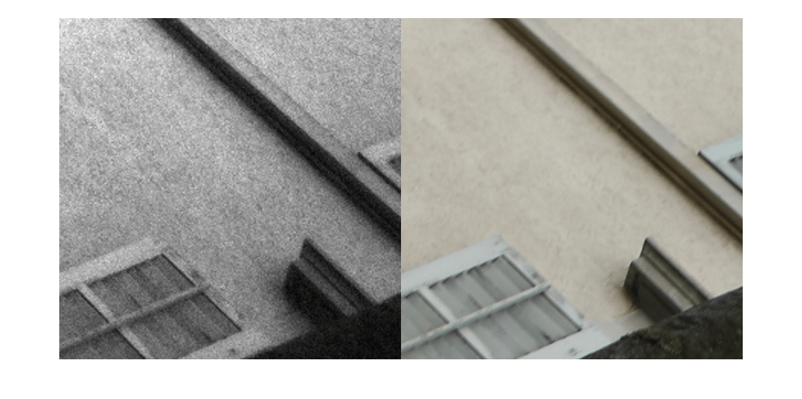
Set Up U-Net Network Layers
This example uses a variation of the U-Net network. In U-Net, the initial series of convolutional layers are interspersed with max pooling layers, successively decreasing the resolution of the input image. These layers are followed by a series of convolutional layers interspersed with upsampling operators, successively increasing the resolution of the input image. The name U-Net comes from the fact that the network can be drawn with a symmetric shape like the letter U.
This example uses a simple U-Net architecture with two modifications. First, the network replaces the final transposed convolution operation with a custom pixel shuffle upsampling (also known as a depth-to-space) operation. Second, the network uses a custom hyperbolic tangent activation layer as the final layer in the network.
Pixel Shuffle Upsampling
Convolution followed by pixel shuffle upsampling can define subpixel convolution for super resolution applications. Subpixel convolution prevents the checkerboard artifacts that can arise from transposed convolution [6]. Because the model needs to map H/2-by-W/2-by-4 RAW inputs to W-by-H-by-3 RGB outputs, the final upsampling stage of the model can be thought of similarly to super resolution where the number of spatial samples grows from the input to the output.
The figure shows how pixel shuffle upsampling works for a 2-by-2-by-4 input. The first two dimensions are spatial dimensions and the third dimension is a channel dimension. In general, pixel shuffle upsampling by a factor of S takes an H-by-W-by-C input and yields an S*H-by-S*W-by- output.

The pixel shuffle function grows the spatial dimensions of the output by mapping information from channel dimensions at a given spatial location into S-by*-S* spatial blocks in the output in which each channel contributes to a consistent spatial position relative to its neighbors during upsampling.
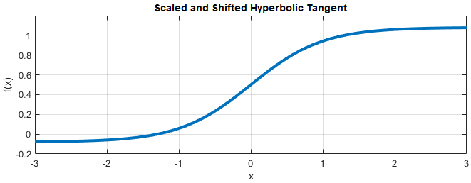
Scaled and Hyperbolic Tangent Activation
A hyperbolic tangent activation layer applies the tanh function on the layer inputs. This example uses a scaled and shifted version of the tanh function, which encourages but does not strictly enforce that the RGB network outputs are in the range [0, 1].
Create U-Net
Create layers of the initial subnetwork.
inputSize = [256 256 4];
initialLayer = imageInputLayer(inputSize,Normalization="zerocenter",Name="ImageInputLayer");
Add layers of the first encoding subnetwork. The first encoder has 32 convolutional filters.
numEncoderStages = 4;
numFiltersFirstEncoder = 32;
encoderNamePrefix = "Encoder-Stage-";

encoderLayers = [
    convolution2dLayer([3 3],numFiltersFirstEncoder,Padding="same", ...
        WeightsInitializer="narrow-normal",Name=encoderNamePrefix+"1-Conv-1")
    leakyReluLayer(0.2,Name=encoderNamePrefix+"1-ReLU-1")
    convolution2dLayer([3 3],numFiltersFirstEncoder,Padding="same", ...
        WeightsInitializer="narrow-normal",Name=encoderNamePrefix+"1-Conv-2")
    leakyReluLayer(0.2,Name=encoderNamePrefix+"1-ReLU-2")
    maxPooling2dLayer([2 2],Stride=[2 2],Name=encoderNamePrefix+"1-MaxPool")
    ];
Add layers of additional encoding subnetworks. These subnetworks add channel-wise instance normalization after each convolutional layer using a groupNormalizationLayer. Each encoder subnetwork has twice the number of filters as the previous encoder subnetwork.
cnIdx = 1;
for stage = 2:numEncoderStages

    numFilters = numFiltersFirstEncoder*2^(stage-1);
    layerNamePrefix = encoderNamePrefix+num2str(stage);

    encoderLayers = [
        encoderLayers
        convolution2dLayer([3 3],numFilters,Padding="same", ...
            WeightsInitializer="narrow-normal",Name=layerNamePrefix+"-Conv-1")
        groupNormalizationLayer("channel-wise",Name="cn"+num2str(cnIdx))
        leakyReluLayer(0.2,Name=layerNamePrefix+"-ReLU-1")
        convolution2dLayer([3 3],numFilters,Padding="same", ...
            WeightsInitializer="narrow-normal",Name=layerNamePrefix+"-Conv-2")
        groupNormalizationLayer("channel-wise",Name="cn"+num2str(cnIdx+1))
        leakyReluLayer(0.2,Name=layerNamePrefix+"-ReLU-2")
        maxPooling2dLayer([2 2],Stride=[2 2],Name=layerNamePrefix+"-MaxPool")
        ];

    cnIdx = cnIdx + 2;
end
Add bridge layers. The bridge subnetwork has twice the number of filters as the final encoder subnetwork and first decoder subnetwork.
numFilters = numFiltersFirstEncoder*2^numEncoderStages;
bridgeLayers = [
    convolution2dLayer([3 3],numFilters,Padding="same", ...
        WeightsInitializer="narrow-normal",Name="Bridge-Conv-1")
    groupNormalizationLayer("channel-wise",Name="cn7")
    leakyReluLayer(0.2,Name="Bridge-ReLU-1")
    convolution2dLayer([3 3],numFilters,Padding="same", ...
        WeightsInitializer="narrow-normal",Name="Bridge-Conv-2")
    groupNormalizationLayer("channel-wise",Name="cn8")
    leakyReluLayer(0.2,Name="Bridge-ReLU-2")];
Add layers of the first three decoder subnetworks.
numDecoderStages = 4;
cnIdx = 9;
decoderNamePrefix = "Decoder-Stage-";

decoderLayers = [];
for stage = 1:numDecoderStages-1

    numFilters = numFiltersFirstEncoder*2^(numDecoderStages-stage);
    layerNamePrefix = decoderNamePrefix+num2str(stage);

    decoderLayers = [
        decoderLayers
        transposedConv2dLayer([3 3],numFilters,Stride=[2 2],Cropping="same", ...
            WeightsInitializer="narrow-normal",Name=layerNamePrefix+"-UpConv")
        leakyReluLayer(0.2,Name=layerNamePrefix+"-UpReLU")
        depthConcatenationLayer(2,Name=layerNamePrefix+"-DepthConcatenation")
        convolution2dLayer([3 3],numFilters,Padding="same", ...
            WeightsInitializer="narrow-normal",Name=layerNamePrefix+"-Conv-1")
        groupNormalizationLayer("channel-wise",Name="cn"+num2str(cnIdx))
        leakyReluLayer(0.2,Name=layerNamePrefix+"-ReLU-1")
        convolution2dLayer([3 3],numFilters,Padding="same", ...
            WeightsInitializer="narrow-normal",Name=layerNamePrefix+"-Conv-2")
        groupNormalizationLayer("channel-wise",Name="cn"+num2str(cnIdx+1))
        leakyReluLayer(0.2,Name=layerNamePrefix+"-ReLU-2")
        ];

    cnIdx = cnIdx + 2;
end
Add layers of the last decoder subnetwork. This subnetwork excludes the channel-wise instance normalization performed by the other decoder subnetworks. Each decoder subnetwork has half the number of filters as the previous subnetwork.
numFilters = numFiltersFirstEncoder;
layerNamePrefix = decoderNamePrefix+num2str(stage+1);

decoderLayers = [
    decoderLayers
    transposedConv2dLayer([3 3],numFilters,Stride=[2 2],Cropping="same", ...
       WeightsInitializer="narrow-normal",Name=layerNamePrefix+"-UpConv")
    leakyReluLayer(0.2,Name=layerNamePrefix+"-UpReLU")
    depthConcatenationLayer(2,Name=layerNamePrefix+"-DepthConcatenation")
    convolution2dLayer([3 3],numFilters,Padding="same", ...
        WeightsInitializer="narrow-normal",Name=layerNamePrefix+"-Conv-1")
    leakyReluLayer(0.2,Name=layerNamePrefix+"-ReLU-1")
    convolution2dLayer([3 3],numFilters,Padding="same", ...
        WeightsInitializer="narrow-normal",Name=layerNamePrefix+"-Conv-2")
    leakyReluLayer(0.2,Name=layerNamePrefix+"-ReLU-2")];
Add the final layers of the U-Net. The pixel shuffle layer moves from the H/2-by-W/2-by-12 channel size of the activations from the final convolution to H-by-W-by-3 channel activations using pixel shuffle upsampling. The final layer encourages outputs to the desired range [0, 1] using a hyperbolic tangent function.
finalLayers = [
    convolution2dLayer([3 3],12,Padding="same",WeightsInitializer="narrow-normal", ...
       Name="Decoder-Stage-4-Conv-3")
    pixelShuffleLayer("pixelShuffle",2)
    tanhScaledAndShiftedLayer("tanhActivation")];

layers = [initialLayer;encoderLayers;bridgeLayers;decoderLayers;finalLayers];
net = dlnetwork(layers,Initialize=false);
Connect layers of the encoding and decoding subnetworks.
net = connectLayers(net,"Encoder-Stage-1-ReLU-2", ...
    "Decoder-Stage-4-DepthConcatenation/in2");
net = connectLayers(net,"Encoder-Stage-2-ReLU-2", ...
    "Decoder-Stage-3-DepthConcatenation/in2");
net = connectLayers(net,"Encoder-Stage-3-ReLU-2", ...
    "Decoder-Stage-2-DepthConcatenation/in2");
net = connectLayers(net,"Encoder-Stage-4-ReLU-2", ...
    "Decoder-Stage-1-DepthConcatenation/in2");
Load the Feature Extraction Network
This function modifies a pretrained VGG-16 deep neural network to extract image features at various layers. These multilayer features are used to compute content loss.
To get a pretrained VGG-16 network, install vgg16 (Deep Learning Toolbox). If you do not have the required support package installed, then the software provides a download link.
To make the VGG-16 network suitable for feature extraction, use the layers up to "relu5_3".
vggNet = pretrainedEncoderNetwork("vgg16",4);Define Loss Functions
The overall loss is a weighted sum of two losses: mean of absolute error (MAE) loss and content loss. The content loss is weighted such that the MAE loss and content loss contribute approximately equally to the overall loss:
The MAE loss penalizes the distance between samples of the network predictions and samples of the target image. is often a better choice than for image processing applications because it can help reduce blurring artifacts [4]. This loss is implemented using the maeLoss helper function defined in the Supporting Functions section of this example.
The content loss helps the network learn both high-level structural content and low-level edge and color information. The loss function calculates a weighted sum of the mean square error (MSE) between predictions and targets for each activation layer. This loss is implemented using the contentLoss helper function defined in the Supporting Functions section of this example.
Calculate Content Loss Weight Factor
Calculate the weight factor for a sample batch of training data such that the MAE loss is equal to the weighted content loss.
Preview a batch of training data, which consists of pairs of RAW network inputs and RGB target outputs.
trainingBatch = preview(dsTrainAug);
networkInput = dlarray((trainingBatch{1,1}),"SSC");
targetOutput = dlarray((trainingBatch{1,2}),"SSC");
Predict the response of the untrained U-Net network using the forward (Deep Learning Toolbox) function.
net = initialize(net,networkInput);
predictedOutput = forward(net,networkInput);
Calculate the MAE and content losses between the predicted and target RGB images.
sampleMAELoss = maeLoss(predictedOutput,targetOutput);
sampleContentLoss = contentLoss(vggNet,predictedOutput,targetOutput);
Calculate the weight factor.
weightContent = sampleMAELoss/sampleContentLoss;
Specify Training Options
Define the training options to control aspects of Adam optimization. Train for 20 epochs.
options = trainingOptions("adam",...
    InitialLearnRate=5e-5,...
    MaxEpochs=20,...
    Plots="training-progress",...
    Shuffle="every-epoch",...
    MiniBatchSize=8,...
    InputDataFormats="SSCB",...
    TargetDataFormats="SSCB");
Train Network or Download Pretrained Network
By default, the example downloads a pretrained version of the RAW-to-RGB network by using the downloadTrainedNetwork helper function. The pretrained network enables you to run the entire example without waiting for training to complete.
To train the network, set the doTraining variable in the following code to true. Train the neural network using the trainnet (Deep Learning Toolbox) function. Use the custom loss function lossFcn, which is defined at the end of the example. By default, the trainnet function uses a GPU if one is available. Training on a GPU requires a Parallel Computing Toolbox™ license and a supported GPU device. For information on supported devices, see GPU Computing Requirements (Parallel Computing Toolbox). Otherwise, the trainnet function uses the CPU. To specify the execution environment, use the ExecutionEnvironment training option. Training takes about 88 hours on an NVIDIA™ Titan RTX GPU.
doTraining = false;
if doTraining
    net = trainnet(dsTrainAug,net,@(Y,T) lossFcn(Y,T,vggNet,weightContent),options);
    modelDateTime = string(datetime("now",Format="yyyy-MM-dd-HH-mm-ss"));
    save(fullfile(dataDir,"trainedRAWToRGBNet-"+modelDateTime+".mat"),"net");
else
    trainedNet_url = "https://ssd.mathworks.com/supportfiles"+ ...
        "/vision/data/trainedRAWToRGBNet.mat";
    downloadTrainedNetwork(trainedNet_url,dataDir);
    load(fullfile(dataDir,"trainedRAWToRGBNet.mat"));
end
Downloading pretrained network.
This can take several minutes to download...
Done.
Calculate Image Quality Metrics
Reference-based quality metrics such as MSSIM or PSNR enable a quantitative measure of image quality. You can calculate the MSSIM and PSNR of the patched test images because they are spatially registered and the same size.
Iterate through the test set of patched images using a minibatchqueue object.
patchTestSet = combine(dsTestRAW,dsTestRGB);
testPatchQueue = minibatchqueue(patchTestSet, ...
    MiniBatchSize=16,MiniBatchFormat="SSCB");
Iterate through the test set and calculate the MSSIM and PSNR for each test image using the multissim and psnr functions. Calculate the MSSIM for color images by using a mean of the metric for each color channel as an approximation because the metric is not well defined for multi-channel inputs.
totalMSSIM = 0;
totalPSNR = 0;
while hasdata(testPatchQueue)
    [inputRAW,targetRGB] = next(testPatchQueue);
    outputRGB = forward(net,inputRAW);
    targetRGB = targetRGB ./ 255;
    mssimOut = sum(mean(multissim(outputRGB,targetRGB),3),4);
    psnrOut = sum(psnr(outputRGB,targetRGB),4);
    totalMSSIM = totalMSSIM + mssimOut;
    totalPSNR = totalPSNR + psnrOut;
end
Calculate the mean MSSIM and mean PSNR over the test set. This result is consistent with the similar U-Net approach from [3] for mean MSSIM and competitive with the PyNet approach in [3] in mean PSNR. The differences in loss functions and use of pixel shuffle upsampling compared to [3] likely account for these differences.
numObservations = dsTestRGB.numpartitions;
meanMSSIM = totalMSSIM / numObservations
meanMSSIM =
  1(S) × 1(S) × 1(C) × 1(B) single gpuArray dlarray

    0.8417
meanPSNR = totalPSNR / numObservations
meanPSNR =
  1(S) × 1(S) × 1(C) × 1(B) single gpuArray dlarray

   21.1001
Evaluate Trained Image Processing Pipeline on Full-Sized Images
Because of sensor differences between the phone camera and DSLR used to acquire the full-resolution test images, the scenes are not registered and are not the same size. Reference-based comparison of the full-resolution images from the network and the DSLR ISP is difficult. However, a qualitative comparison of the images is useful because a goal of image processing is to create an aesthetically pleasing image.
Create an image datastore that contains full-sized RAW images acquired by a phone camera.
testImageDir = fullfile(dataDir,"test");
testImageDirRAW = "huawei_full_resolution";
dsTestFullRAW = imageDatastore(fullfile(testImageDir,testImageDirRAW));
Get the names of the image files in the full-sized RAW test set.
targetFilesToInclude = extractAfter(string(dsTestFullRAW.Files), ...
    fullfile(testImageDirRAW,filesep));
targetFilesToInclude = extractBefore(targetFilesToInclude,".png");
Preprocess the RAW data by converting the data to the form expected by the network using the transform function. The transform function processes the data using the operations specified in the preprocessRAWDataForRAWToRGB helper function. The helper function is attached to the example as a supporting file.
dsTestFullRAW = transform(dsTestFullRAW,@preprocessRAWDataForRAWToRGB);
Create an image datastore that contains full-sized RGB test images captured from the high-end DSLR. The Zurich RAW-to-RGB data set contains more full-sized RGB images than RAW images, so include only the RGB images with a corresponding RAW image.
dsTestFullRGB = imageDatastore(fullfile(dataDir,"full_resolution","canon"));
dsTestFullRGB.Files = dsTestFullRGB.Files( ...
    contains(dsTestFullRGB.Files,targetFilesToInclude));
Read in the target RGB images, then display a montage of the first few images.
targetRGB = readall(dsTestFullRGB);
montage(targetRGB,Size=[5 2],Interpolation="bilinear")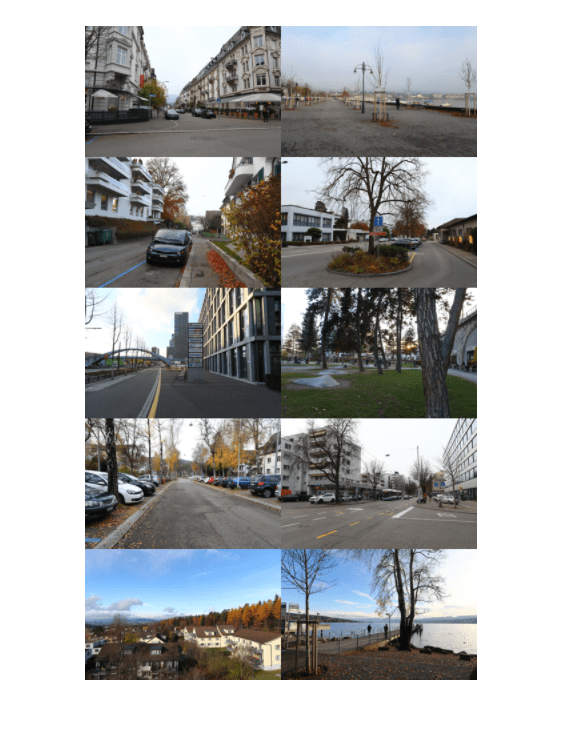
Iterate through the test set of full-sized images using a minibatchqueue object. If you have a supported GPU device with sufficient memory to process full-resolution images, then you can run prediction on the GPU by specifying the output environment as "gpu".
testQueue = minibatchqueue(dsTestFullRAW,MiniBatchSize=1, ...
    MiniBatchFormat="SSCB",OutputEnvironment="cpu");
For each full-sized RAW test image, predict the output RGB image by calling forward (Deep Learning Toolbox) on the network.
outputSize = 2*size(preview(dsTestFullRAW),[1 2]);
outputImages = zeros([outputSize,3,dsTestFullRAW.numpartitions],"uint8");

idx = 1;
while hasdata(testQueue)
    inputRAW = next(testQueue);
    rgbOut = forward(net,inputRAW);
    rgbOut = gather(extractdata(rgbOut));
    outputImages(:,:,:,idx) = im2uint8(rgbOut);
    idx = idx+1;
end
Get a sense of the overall output by looking at a montage view. The network produces images that are aesthetically pleasing, with similar characteristics.
montage(outputImages,Size=[5 2],Interpolation="bilinear")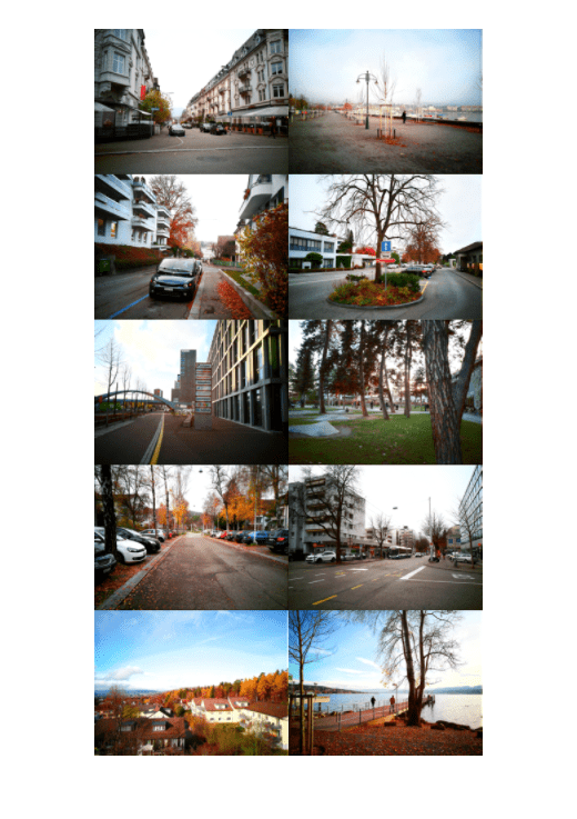
Compare one target RGB image with the corresponding image predicted by the network. The network produces colors which are more saturated than the target DSLR images. Although the colors from the simple U-Net architecture are not the same as the DSLR targets, the images are still qualitatively pleasing in many cases.
imgIdx = 1;
imTarget = targetRGB{imgIdx};
imPredicted = outputImages(:,:,:,imgIdx);
montage({imTarget,imPredicted},Interpolation="bilinear")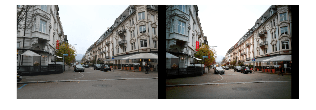
To improve the performance of the RAW-to-RGB network, a network architecture would learn detailed localized spatial features using multiple scales from global features that describe color and contrast [3].
Supporting Functions
Loss Function
The loss function computes the overall loss given outputs from the network, Y, and the corresponding target images, T. Pass additional inputs vggNet and weightContent to the loss using an anonymous function in the call to trainnet.
function loss = lossFcn(Y,T,vggNet,weightContent)
    lossMAE = maeLoss(Y,T);
    lossContent = contentLoss(vggNet,Y,T);
    loss = lossMAE + weightContent.*lossContent;
end
Mean Absolute Error Loss Function
The helper function maeLoss computes the mean absolute error between network predictions, Y, and target images, T.
function loss = maeLoss(Y,T)
    loss = mean(abs(Y-T),"all");
end
Content Loss Function
The helper function contentLoss calculates a weighted sum of the MSE between network predictions, Y, and target images, T, for each activation layer. The contentLoss helper function calculates the MSE for each activation layer using the mseLoss helper function. Weights are selected such that the loss from each activation layers contributes roughly equally to the overall content loss.
function loss = contentLoss(net,Y,T)

    layers = ["relu1_1","relu1_2","relu2_1","relu2_2", ...
        "relu3_1","relu3_2","relu3_3","relu4_1"];
    [T1,T2,T3,T4,T5,T6,T7,T8] = forward(net,T,Outputs=layers);
    [X1,X2,X3,X4,X5,X6,X7,X8] = forward(net,Y,Outputs=layers);

    l1 = mseLoss(X1,T1);
    l2 = mseLoss(X2,T2);
    l3 = mseLoss(X3,T3);
    l4 = mseLoss(X4,T4);
    l5 = mseLoss(X5,T5);
    l6 = mseLoss(X6,T6);
    l7 = mseLoss(X7,T7);
    l8 = mseLoss(X8,T8);

    layerLosses = [l1 l2 l3 l4 l5 l6 l7 l8];
    weights = [1 0.0449 0.0107 0.0023 6.9445e-04 2.0787e-04 2.0118e-04 6.4759e-04];
    loss = sum(layerLosses.*weights);
end
Mean Square Error Loss Function
The helper function mseLoss computes the MSE between network predictions, Y, and target images, T.
function loss = mseLoss(Y,T)
    loss = mean((Y-T).^2,"all");
end
References
1) Sumner, Rob. "Processing RAW Images in MATLAB". May 19, 2014. https://rcsumner.net/raw_guide/RAWguide.pdf.
2) Chen, Chen, Qifeng Chen, Jia Xu, and Vladlen Koltun. “Learning to See in the Dark.” ArXiv:1805.01934 [Cs], May 4, 2018. https://arxiv.org/abs/1805.01934.
3) Ignatov, Andrey, Luc Van Gool, and Radu Timofte. “Replacing Mobile Camera ISP with a Single Deep Learning Model.” ArXiv:2002.05509 [Cs, Eess], February 13, 2020. http://arxiv.org/abs/2002.05509. Project Website.
4) Zhao, Hang, Orazio Gallo, Iuri Frosio, and Jan Kautz. “Loss Functions for Neural Networks for Image Processing.” ArXiv:1511.08861 [Cs], April 20, 2018. http://arxiv.org/abs/1511.08861.
5) Johnson, Justin, Alexandre Alahi, and Li Fei-Fei. “Perceptual Losses for Real-Time Style Transfer and Super-Resolution.” ArXiv:1603.08155 [Cs], March 26, 2016. https://arxiv.org/abs/1603.08155.
6) Shi, Wenzhe, Jose Caballero, Ferenc Huszár, Johannes Totz, Andrew P. Aitken, Rob Bishop, Daniel Rueckert, and Zehan Wang. “Real-Time Single Image and Video Super-Resolution Using an Efficient Sub-Pixel Convolutional Neural Network.” ArXiv:1609.05158 [Cs, Stat], September 23, 2016. https://arxiv.org/abs/1609.05158.
See Also
imageDatastore | transform | combine | dlnetwork (Deep Learning Toolbox) | trainingOptions (Deep Learning Toolbox) | trainnet (Deep Learning Toolbox) | forward (Deep Learning Toolbox)
Topics
- Brighten Extremely Dark Images Using Deep Learning
- Preprocess Images for Deep Learning (Deep Learning Toolbox)
- Datastores for Deep Learning (Deep Learning Toolbox)
- List of Deep Learning Layers (Deep Learning Toolbox)