Augment Images for Deep Learning
This example shows how you can perform common kinds of randomized image augmentation. Common types of image transformations include image warping and cropping, color adjustments, and adding synthetic distortions such as noise and blur.
Image augmentation is a type of image preprocessing that enables you to effectively increase the amount of training and test data. Augmentation also enables you to train networks to be invariant to distortions in image data. For example, you can add randomized rotations to input images so that a network is invariant to the presence of rotation in input images. In practical deep learning problems, the image augmentation pipeline typically combines multiple operations.
You can implement common types of image augmentation by using functions in Image Processing Toolbox. This topic demonstrates common types of transformations that you can apply to images:
Datastores are a convenient way to augment collections of images. You can use the transform function to apply any combination of functions to images in datastores. You can use the combine function to apply identical augmentations to pairs of images in datastores. This topic shows how to apply augmentation to image data in datastores for image classification and image-to-image regression.
You can use augmented training data to train a network. For an example of training a network using augmented images, see Prepare Datastore for Image-to-Image Regression (Deep Learning Toolbox).
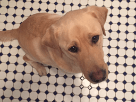
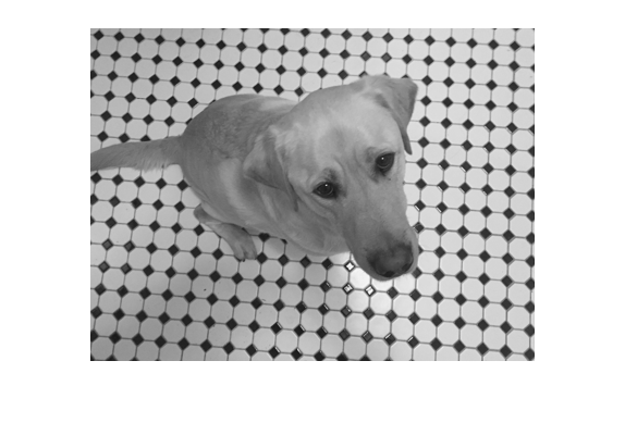
Read and display a sample image. To compare the effect of the different types of image augmentation, each transformation uses the same input image.
imOriginal = imresize(imread("kobi.png"),0.25);
imageshow(imOriginal)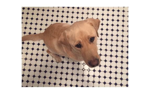
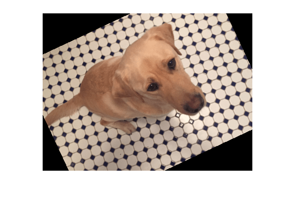
Random Image Warping Transformations
The randomAffine2d function creates a randomized 2-D affine transformation from a combination of rotation, translation, scale (resizing), reflection, and shear. You can specify which transformations to include and the range of transformation parameters. If you specify the range as a 2-element numeric vector, then randomAffine2d selects the value of a parameter from a uniform probability distribution over the specified interval. For more control of the range of parameter values, you can specify the range using a function handle.
Control the spatial bounds and resolution of the warped image created by imwarp by using the affineOutputView function.
Rotation
Create a randomized rotation transformation that rotates the input image by an angle selected randomly from the range [-45, 45] degrees.
tform = randomAffine2d(Rotation=[-45 45]);
outputView = affineOutputView(size(imOriginal),tform);
imAugmented = imwarp(imOriginal,tform,OutputView=outputView);
imageshow(imAugmented)
Translation
Create a translation transformation that shifts the input image horizontally and vertically by a distance selected randomly from the range [-50, 50] pixels.
tform = randomAffine2d(XTranslation=[-50 50],YTranslation=[-50 50]);
outputView = affineOutputView(size(imOriginal),tform);
imAugmented = imwarp(imOriginal,tform,OutputView=outputView);
imageshow(imAugmented)
Scale
Create a scale transformation that resizes the input image using a scale factor selected randomly from the range [1.2, 1.5]. This transformation resizes the image by the same factor in the horizontal and vertical directions.
tform = randomAffine2d(Scale=[1.2,1.5]);
outputView = affineOutputView(size(imOriginal),tform);
imAugmented = imwarp(imOriginal,tform,OutputView=outputView);
imageshow(imAugmented)
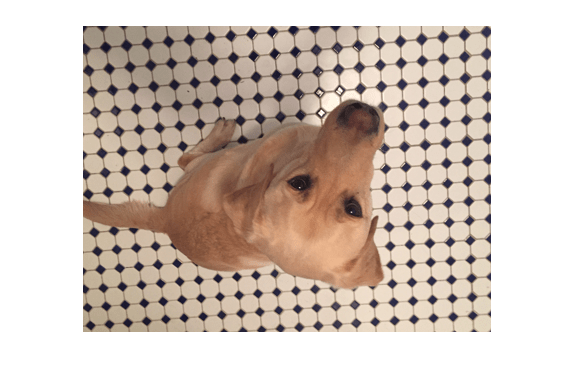
Reflection
Create a reflection transformation that flips the input image with 50% probability in each dimension.
tform = randomAffine2d(XReflection=true,YReflection=true);
outputView = affineOutputView(size(imOriginal),tform);
imAugmented = imwarp(imOriginal,tform,OutputView=outputView);
imageshow(imAugmented)
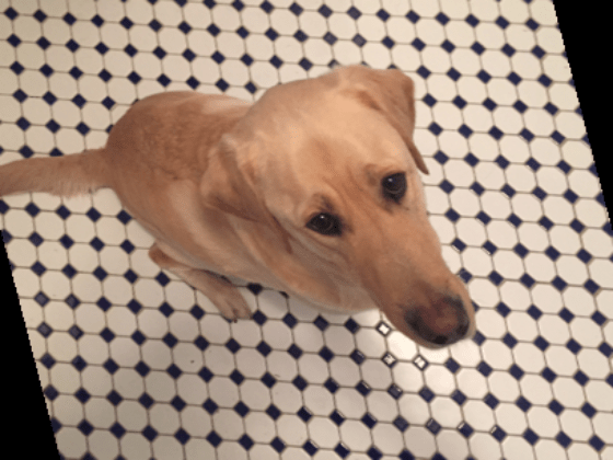
Shear
Create a horizontal shear transformation with the shear angle selected randomly from the range [-30, 30].
tform = randomAffine2d(XShear=[-30 30]);
outputView = affineOutputView(size(imOriginal),tform);
imAugmented = imwarp(imOriginal,tform,OutputView=outputView);
imageshow(imAugmented)
Control Range of Transformation Parameters Using Custom Selection Function
In the preceding transformations, the range of transformation parameters was specified by two-element numeric vectors. For more control of the range of the transformation parameters, specify a function handle instead of a numeric vector. The function handle takes no input arguments and yields a valid value for each parameter.
For example, this code selects a rotation angle from a discrete set of 90 degree rotation angles.
angles = 0:90:270;
tform = randomAffine2d(Rotation=@() angles(randi(4)));
outputView = affineOutputView(size(imOriginal),tform);
imAugmented = imwarp(imOriginal,tform,OutputView=outputView);
imageshow(imAugmented)
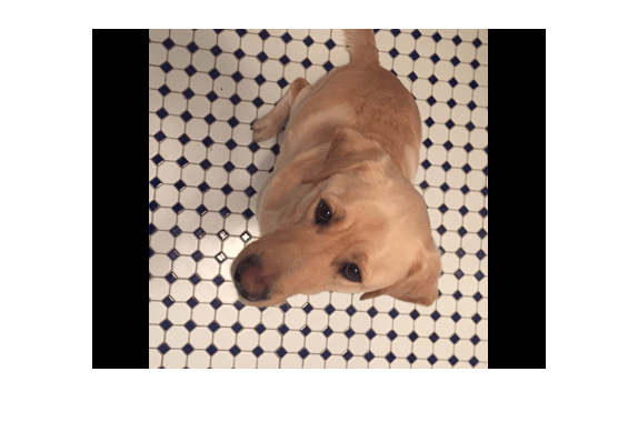
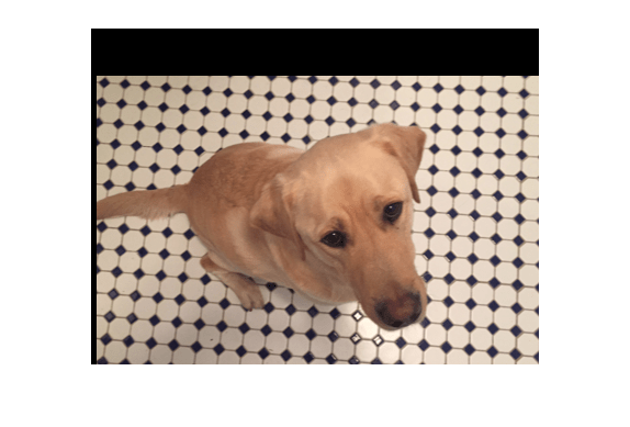
Control Fill Value
When you warp an image using a geometric transformation, pixels in the output image can map to a location outside the bounds of the input image. In that case, imwarp assigns a fill value to those pixels in the output image. By default, imwarp selects black as the fill value. You can change the fill value by specifying the FillValues name-value argument.
Create a random rotation transformation, then apply the transformation and specify a gray fill value.
tform = randomAffine2d(Rotation=[-45 45]);
outputView = affineOutputView(size(imOriginal),tform);
imAugmented = imwarp(imOriginal,tform,OutputView=outputView, ...
    FillValues=[128 128 128]);
imageshow(imAugmented)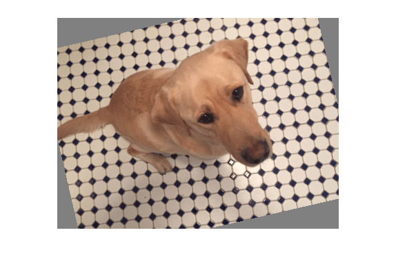
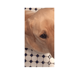
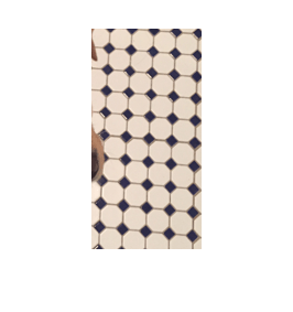
Cropping Transformations
To create output images of a desired size, use the randomWindow2d and centerCropWindow2d functions. Be careful to select a window that includes the desired content in the image.
Specify the desired size of the cropped region as a 2-element vector of the form [height, width].
targetSize = [200,100];
Crop the image to the target size from the center of the image.
win = centerCropWindow2d(size(imOriginal),targetSize);
imCenterCrop = imcrop(imOriginal,win);
imageshow(imCenterCrop)
Crop the image to the target size from a random location in the image.
win = randomWindow2d(size(imOriginal),targetSize);
imRandomCrop = imcrop(imOriginal,win);
imageshow(imRandomCrop)
Color Transformations
You can randomly adjust the hue, saturation, brightness, and contrast of a color image by using the jitterColorHSV function. You can specify which color transformations are included and the range of transformation parameters.
You can randomly adjust the brightness and contrast of grayscale images by using basic math operations.
Hue Jitter
Hue specifies the shade of color, or a color's position on a color wheel. As hue varies from 0 to 1, colors vary from red through yellow, green, cyan, blue, purple, magenta, and back to red. Hue jitter shifts the apparent shade of colors in an image.
Adjust the hue of the input image by a small positive offset selected randomly from the range [0.05, 0.15]. Colors that were red now appear more orange or yellow, colors that were orange appear yellow or green, and so on.
imJittered = jitterColorHSV(imOriginal,Hue=[0.05 0.15]);
montage({imOriginal,imJittered})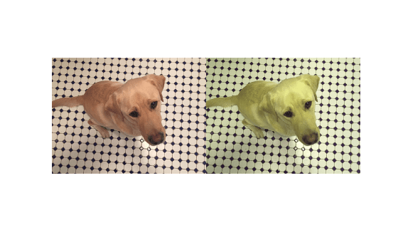
Saturation Jitter
Saturation is the purity of color. As saturation varies from 0 to 1, hues vary from gray (indicating a mixture of all colors) to a single pure color. Saturation jitter shifts how dull or vibrant colors are.
Adjust the saturation of the input image by an offset selected randomly from the range [-0.4, -0.1]. The colors in the output image appear more muted, as expected when the saturation decreases.
imJittered = jitterColorHSV(imOriginal,Saturation=[-0.4 -0.1]);
montage({imOriginal,imJittered})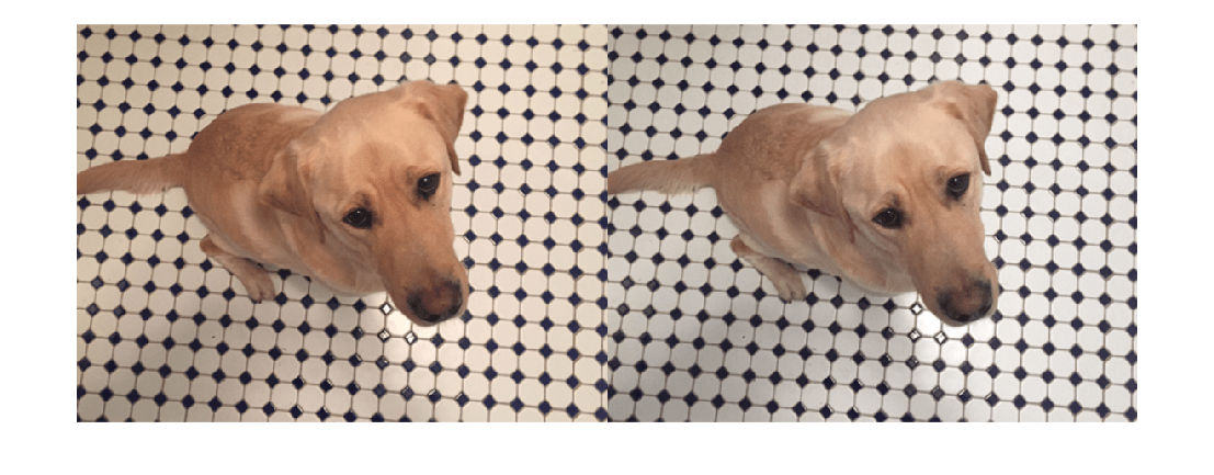
Brightness Jitter
Brightness is the amount of hue. As brightness varies from 0 to 1, colors go from black to white. Brightness jitter shifts the darkness and lightness of an input image.
Adjust the brightness of the input image by an offset selected randomly from the range [-0.3, -0.1]. The image appears darker, as expected when the brightness decreases.
imJittered = jitterColorHSV(imOriginal,Brightness=[-0.3 -0.1]);
montage({imOriginal,imJittered})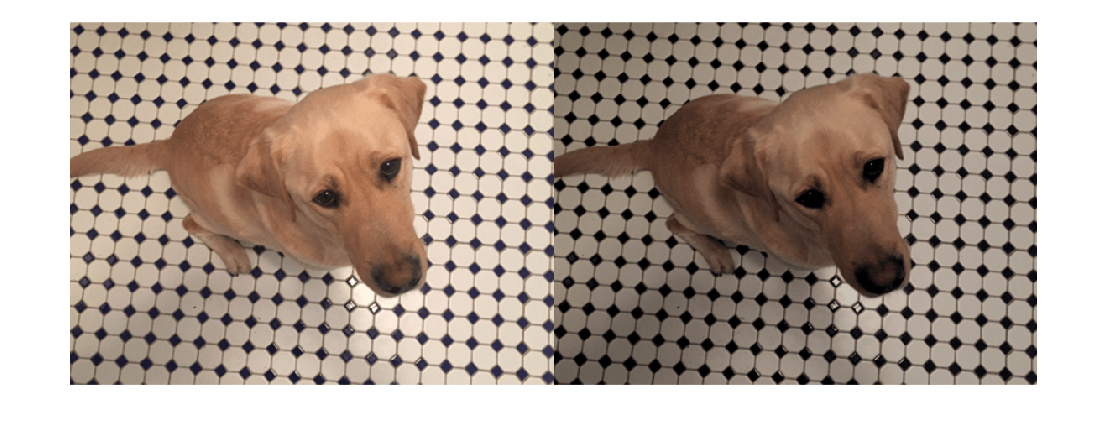
Contrast Jitter
Contrast jitter randomly adjusts the difference between the darkest and brightest regions in an input image.
Adjust the contrast of the input image by a scale factor selected randomly from the range [1.2, 1.4]. The contrast increases, such that shadows become darker and highlights become brighter.
imJittered = jitterColorHSV(imOriginal,Contrast=[1.2 1.4]);
montage({imOriginal,imJittered})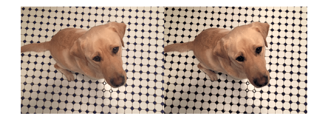
Brightness and Contrast Jitter of Grayscale Images
You can apply randomized brightness and contrast jitter to grayscale images by using basic math operations.
Convert the sample image to grayscale. Specify a random contrast scale factor in the range [0.8, 1] and a random brightness offset in the range [-0.15, 0.15]. Multiply the image by the contrast scale factor, then add the brightness offset.
imGray = im2gray(im2double(imOriginal));
contrastFactor = 1-0.2*rand;
brightnessOffset = 0.3*(rand-0.5);
imJittered = imGray.*contrastFactor + brightnessOffset;
imJittered = im2uint8(imJittered);
montage({imGray,imJittered})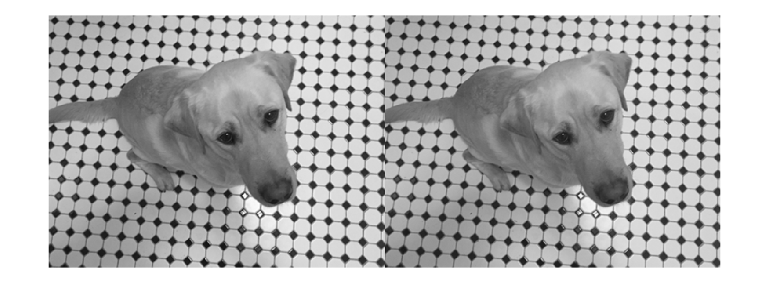
Randomized Color-to-Grayscale
One type of color augmentation randomly removes the color information from an RGB image while preserving the number of channels expected by the network. This code shows a "random grayscale" transformation in which an RGB image is randomly converted with 80% probability to a three channel output image where R == G == B.
desiredProbability = 0.8;
if rand <= desiredProbability
    imJittered = repmat(rgb2gray(imOriginal),[1 1 3]);
end
imageshow(imJittered)
Synthetic Distortion
Use the transform function to apply any combination of Image Processing Toolbox functions to input images. Adding noise and blur are two common image processing operations used in deep learning applications.
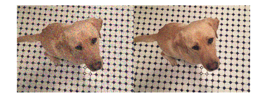
Synthetic Noise
To apply synthetic noise to an input image, use the imnoise function. You can specify which noise model to use, such as Gaussian, Poisson, salt and pepper, and multiplicative noise. You can also specify the strength of the noise.
imSaltAndPepperNoise = imnoise(imOriginal,"salt & pepper",0.1);
imGaussianNoise = imnoise(imOriginal,"gaussian");
montage({imSaltAndPepperNoise,imGaussianNoise})
Synthetic Blur
To apply randomized Gaussian blur to an image, use the imgaussfilt function. You can specify the amount of smoothing.
sigma = 1+5*rand;
imBlurred = imgaussfilt(imOriginal,sigma);
imageshow(imBlurred)

Apply Augmentation to Image Data in Datastores
In practical deep learning problems, the image augmentation pipeline typically combines multiple operations. Datastores are a convenient way to read and augment collections of images.
This section of the example shows how to define data augmentation pipelines that augment datastores in the context of training image classification and image regression problems.
First, create an imageDatastore that contains unprocessed images. The image datastore in this example contains digit images with labels.
digitDatasetPath = fullfile(matlabroot,"toolbox","nnet", ...
    "nndemos","nndatasets","DigitDataset");
imds = imageDatastore(digitDatasetPath, ...
    IncludeSubfolders=true,LabelSource="foldernames");
imds.ReadSize = 6;
Image Classification
In image classification, the classifier should learn that a randomly altered version of an image still represents the same image class. To augment data for image classification, it is sufficient to augment the input images while leaving the corresponding categorical labels unchanged.
Define a helper function, named classificationAugmentationPipeline, that augments images for classification. dataIn and dataOut are two-element cell arrays, where the first element is the network input image and the second element is the categorical label. The function augments input images by applying random Gaussian blur, salt and pepper noise, and randomized scale and rotation.
function [dataOut,info] = classificationAugmentationPipeline(dataIn,info)

dataOut = cell([size(dataIn,1),2]);

for idx = 1:size(dataIn,1)
    temp = dataIn{idx};

    % Add randomized Gaussian blur
    temp = imgaussfilt(temp,1.5*rand);

    % Add salt and pepper noise
    temp = imnoise(temp,"salt & pepper");

    % Add randomized rotation and scale
    tform = randomAffine2d(Scale=[0.95,1.05],Rotation=[-30 30]);
    outputView = affineOutputView(size(temp),tform);
    temp = imwarp(temp,tform,OutputView=outputView);

    % Form a two-element cell array with the input image and expected response
    dataOut(idx,:) = {temp,info.Label(idx)};
end

end
Augment images in the pristine image datastore by using the transform function and specifying the transformation function as the classificationAugmentationPipeline helper function.
dsTrain = transform(imds,@classificationAugmentationPipeline, ...
    IncludeInfo=true);
Visualize a sample of the output coming from the augmented pipeline.
dataPreview = preview(dsTrain);
montage(dataPreview(:,1))
title("Augmented Images for Image Classification")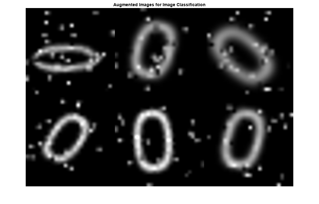
Image Regression
Image augmentation for image-to-image regression is more complicated because you must apply identical geometric transformations to the input and response images. Associate pairs of input and response images by using the combine function. Transform one or both images in each pair by using the transform function.
Combine two identical copies of the image datastore imds. When data is read from the combined datastore, image data is returned in a two-column cell array, where the first column represents network input images and the second column contains network responses.
dsCombined = combine(imds,imds);
montage(preview(dsCombined)',Size=[6 2])
title("Combined Input and Response Pairs Before Augmentation")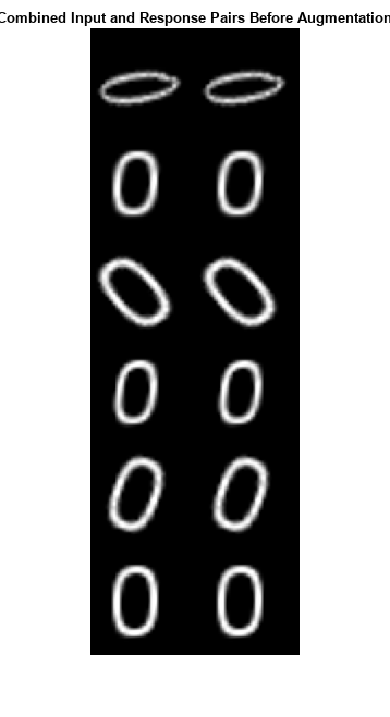
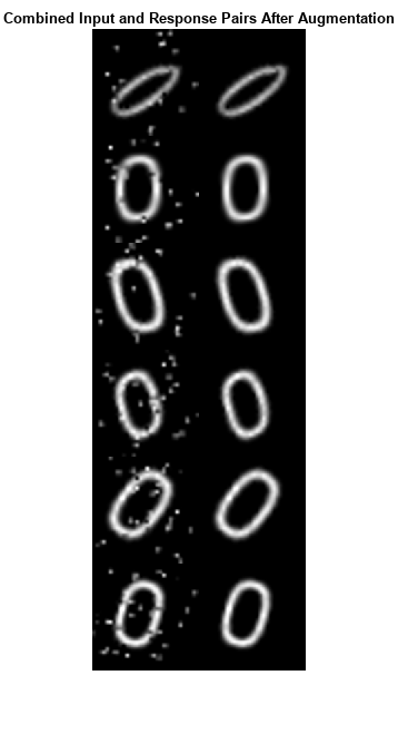
Define a helper function, named imageRegressionAugmentationPipeline, that augments images for image-to-image regression. dataIn and dataOut are two-element cell arrays, where the first element is the network input image and the second element is the network response image. The function augments the network input and response images by performing this series of image processing operations:
Resize the input and response image to 32-by-32 pixels.
Add salt and pepper noise to the input image only.
Create a transformation that has randomized scale and rotation.
Apply the same transformation to the input and response image.
function dataOut = imageRegressionAugmentationPipeline(dataIn)

dataOut = cell([size(dataIn,1),2]);
for idx = 1:size(dataIn,1)

    % Resize images to 32-by-32 pixels and convert to data type single
    inputImage = im2single(imresize(dataIn{idx,1},[32 32]));
    targetImage = im2single(imresize(dataIn{idx,2},[32 32]));

    % Add salt and pepper noise
    inputImage = imnoise(inputImage,"salt & pepper");

    % Add randomized rotation and scale
    tform = randomAffine2d(Scale=[0.9,1.1],Rotation=[-30 30]);
    outputView = affineOutputView(size(inputImage),tform);

    % Use imwarp with the same tform and outputView to augment both images
    % the same way
    inputImage = imwarp(inputImage,tform,OutputView=outputView);
    targetImage = imwarp(targetImage,tform,OutputView=outputView);

    dataOut(idx,:) = {inputImage,targetImage};
end

end
Augment images in the combined image datastore by using the transform function and specifying the transformation function as the imageRegressionAugmentationPipeline helper function.
dsTrain = transform(dsCombined,@imageRegressionAugmentationPipeline);
montage(preview(dsTrain)',Size=[6 2])
title("Combined Input and Response Pairs After Augmentation")