Optimize Monochromatic Camera Lens System for Type 2/3 Sensor

Define Lens Design Parameters

Begin by specifying the target wavelength, in nanometers, for your optical system.

design.Wavelength = optics.constant.Fraunhofer.d;

Configure Optical Layout

Define a four singlet-lens system, with the aperture stop, or diaphragm, positioned centrally to help minimize aberrations.

Specify to include the semi-diameter of the diaphragm as an optimization variable.

design.NumSemiDiameters = 1;

Specify eight radii of curvature to optimize, as each of the four singlet lenses has two refractive surfaces.

design.NumRadius = 4*2;

Specify the number of lens thicknesses to optimize, which corresponds to the number of singlets.

design.NumThickness = 4;

Specify four materials to optimize, one for each lens. Each singlet is modeled with its own glass type, characterized only by its refractive index, Nd. The monochromatic design does not consider chromatic dispersion, characterized by the Abbe number.

design.NumMaterials = 4;

The system consists of six optical elements: four singlets, one diaphragm, and the image plane. This results in five air gaps; four of which are variable, while the last gap is typically fixed by the mechanical mounting, or the flange focal distance.

Specify the number of gaps to optimize as 4.

design.NumGaps = 4;

To model the standard 2/3'' sensor with an active area of 8.8-by-6.6 square millimeters as an image plane, specify the sensor semi-diagonal as 5.5. Units are in millimeters.

design.SensorSemiDiag = 5.5;

Configure Design Ranges

When designing optical systems, your choices are often limited by what is physically possible to manufacture. To ensure your design is both practical and optimized, define range variables for each key parameter. These variable specify the minimum and maximum values allowed during optimization. For example, for this lens design, you set the maximum semi-diameter of all singlets to 10 mm. This ensures the lens fits within a compact, C-mount-compatible housing.

Specify the minimum semi-diameter, as well as the allowable ranges for curvature and thickness, based on your supplier’s capabilities and your project’s budget. Specify these parameters in millimeters.

Note: Very small radii may be automatically excluded if they conflict with the semi-diameter limits.

design.SemidiameterRange     = [3 10];
design.CurvatureRange        = [-1/20 1/20];
design.CenterThicknessRange  = [1 4];

Specify the gap range, in millimeters. The gaps between optical elements are constrained by the Total Track Length (TTL), the thickness range you set above, and any special mounting requirements.

design.GapRange = [0.5 6];

By default, these ranges apply to every instance of the corresponding variable. However, you can customize them for individual elements if needed. For example, you might specify different semi-diameter ranges to create a tapered or symmetric lens profile.

To define a suitable range for the refractive index, Nd, examine the distribution of available values in the glass library using the glassLibrary object. Plot the distribution of refractive index values in the glass library.

gl = glassLibrary;
design.AvailableNds = [gl.Glasses.Nd];
histogram(design.AvailableNds)
xlabel("Nd")
ylabel("Count")

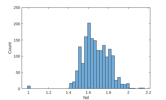
Specify a range of mid-range values from the distribution that fits your application needs.

design.NdRange = [1.5 1.8];

Next, create a list of discrete Nd values within your selected range. During optimization, only these values will be considered.

inRangeInds = design.AvailableNds>=design.NdRange(1) & design.AvailableNds<=design.NdRange(2);
design.AvailableNds = design.AvailableNds(inRangeInds);
disp(numel(design.AvailableNds))

        1339

Configure Design Goals and Weights

To guide the optical system optimization, start by defining your design goals and assigning their relative importance using a structure, goal. Each weight reflects how much that particular goal should influence the optimization, and requires careful tuning and iteration to achieve the best results.

Specify the required focal length, in millimeters, and its weight, which indicates its priority in the optimization process.

goal.FocalLength = 25;
goal.FocalLengthWeight = 5;

Specify the F-number required for your application. You do not set the weight explicitly because the updateSemiDiameters function automatically adjusts the semi-diameters to achieve this F-number based on the current focal length.

goal.FNumber = 4;

Specify the field point goal at three key positions using the fieldPoint function, with higher emphasis on the on-axis field point. Specify the reference frame relative to the image plane using the ReferenceFrame name-value argument. The weights should sum to 1.

goal.FieldPoints = fieldPoint(Position=[0 0; 0 3.8; 0 5],ReferenceFrame="Image");
goal.FieldPointsWeight = [0.6 0.3 0.1];

Specify the spot RMS goal close to the diffraction limit, where the Airy disk radius reaches its first zero.

goal.SpotRMS = 1.22*goal.FNumber*design.Wavelength/1e6;
goal.SpotRMSWeight = 1;

Specify the total length from the first surface to the image plane, and assign a moderate weight.

goal.TTL = 50;
goal.TTLWeight = 0.5;

Create Inputs for Optimization Explorer

To use the Optimization Explorer app to automate design optimization, express your optical system variables as numeric vectors. These vectors define the lower and upper bounds, as well as a starting point for the optimization. This enables the app to handle a wide range of parameter values.

Note: The initial guess, x0, is arbitrary and only used to define the size and structure of the optimization variables. The app uses multiple starting points for the actual optimization.

lb = [...
    repmat(design.SemidiameterRange(1),[1 design.NumSemiDiameters]), ...
    repmat(design.CurvatureRange(1),[1 design.NumRadius]), ...
    repmat(design.CenterThicknessRange(1),[1 design.NumThickness]), ...
    repmat(design.GapRange(1),[1 design.NumGaps]), ...
    repmat(design.NdRange(1),[1 design.NumMaterials])];
ub = [...
    repmat(design.SemidiameterRange(2),[1 design.NumSemiDiameters]), ...
    repmat(design.CurvatureRange(2),[1 design.NumRadius]), ...
    repmat(design.CenterThicknessRange(2),[1 design.NumThickness]), ...
    repmat(design.GapRange(2),[1 design.NumGaps]), ...
    repmat(design.NdRange(2),[1 design.NumMaterials])];
x0 = (ub+lb)/2;

Use the custom x2opsys helper function to generate an optical system from your initial optimization parameter values and your design and goal structures. Use the viewWithInfo helper function to visualize the generated optical system and display the nonoptimized target parameters.

opsys = x2opsys(x0,design,goal);
viewWithInfo(opsys,goal);

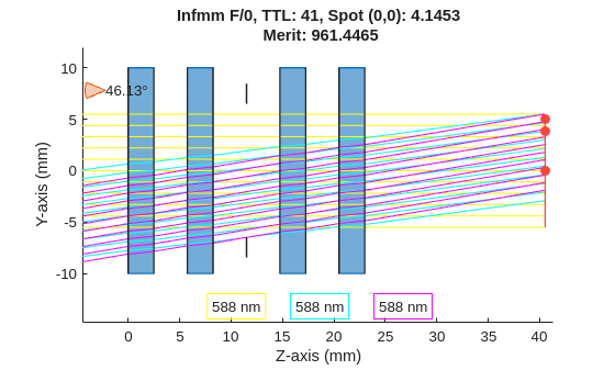
Infmm F/0, TTL: 41, Spot (0,0): 4.1453
 Merit: 961.4465

Define Objective Function

Optimization algorithms require an objective function, a function that takes a set of design parameters in numerical form and returns a value that measures how well a particular design performs. In this example, you can specify the merit function as the objective function using the opticalMeritFunction helper function. This function evaluates the optical system and outputs a vector of merit values. Merit values closer to zero are considered superior.

meritFcn = @(x)opticalMeritFunction(x2opsys(x,design,goal),goal);

Optimize Design Using Optimization Explorer

When running optimization algorithms, random values are often used for initialization and during the optimization process. To ensure your results are repeatable, use the rng function to reset the random number generator to its default state before starting the optimization. If you want to explore different regions of the design space or do not need repeatable results, you can remove this line.

Note: When running in parallel mode, some randomness may persist due to differences in the timing of parallel computations.

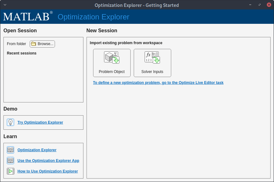
rng("default");

Open the Optimization Explorer app. Alternatively, you can also open the app from the Apps tab of the MATLAB® Toolstrip, under Math, Statistics, and Optimization, by selecting the Optimization Explorer app icon. To get started with the app, see Use Optimization Explorer App (Optimization Toolbox).

optimizationExplorer

In the New Session section of the Getting Started window, select Solver Inputs.

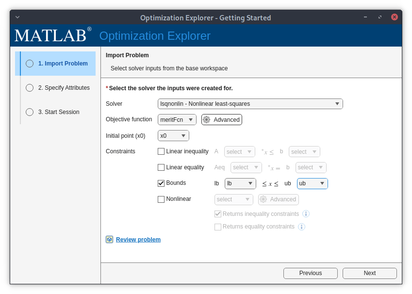
Next, in the Import Problem step, specify these options:

Click Next.

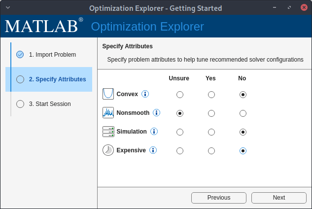
In the Specify Attributes step, set the Nonsmooth attribute to Unsure, as optical optimization problems are typically, but not strictly, nonsmooth. Select No for the remaining attributes to indicate that the problem is not convex, a simulation, or expensive to compute. Click Next.

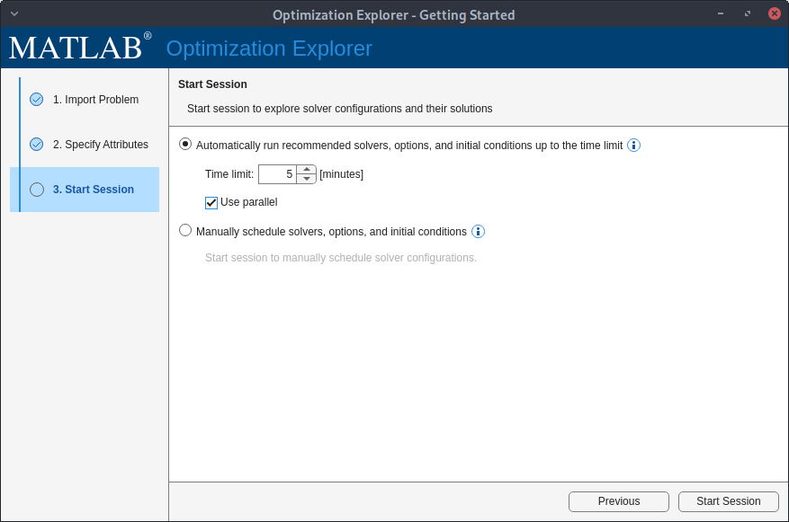
In the Start Session step, select Automatically run recommended solvers, options, and initial conditions up to the time limit, and then specify a small time limit of 5 minutes for the first session only to ensure a correct setup. Select Use parallel if you have access to a parallel computing pool and a Parallel Computing Toolbox™ license. To set up parallel computing for optimization, see Using Parallel Computing in Optimization Toolbox (Optimization Toolbox). Later, you can increase the time limit to probe better designs. To start the optimization session, click Start Session.

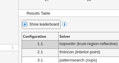
While the app is running, sort the results table in ascending order of the objective value, which is the optical merit function value, by selecting the Show leaderboard button in the Results Table pane. This ensures that the best solution, the solution with the lowest objective value, appears in the first row of the table.

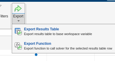
Finally, when the optimization time window is complete, or you have decided the process has converged based on the objective value of each solution displayed in the Results Table, export the sorted table by selecting Export in the app toolstrip, and then Export Results Table. Save the data table as a variable named explorerResultsTable, which is the default variable name.

The explorerResults MAT file, attached to this example as a supporting file, contains the complete optimization results from a session run using a parallel computing environment. The optimization session was run for 20 minutes, the first 10 minutes of which were in Auto mode, and the last 10 minutes of which used manually scheduled local optimization solvers seeded with initial conditions from the solver results of the first 10-minute run. Load the results of this optimization session.

load explorerResults

View Top Four Optimized Designs

Load and explore the top four optical designs, displaying each one along with its key performance metrics. The values in explorerResultsTable are already sorted by the objective function, the merit value, in ascending order it was exported after selecting Show leaderboard in Optimization Explorer. This means the design with the lowest, or best, merit value is at the top of the table.

Display 2-D visualizations of the optimized optical designs in ascending order, from the fourth best to the best performing design. Use the x2opsys helper function to create an optical system object for each set of optimized parameters, and the viewWithInfo helper function to plot each system.

for sInd = 4:-1:1
    xopt = explorerResultsTable.Solution{sInd};
    opsysopt = x2opsys(xopt,design,goal);
    figure
    viewWithInfo(opsysopt,goal)
end

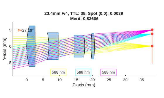
23.4mm F/4, TTL: 38, Spot (0,0): 0.0039
 Merit: 0.83606

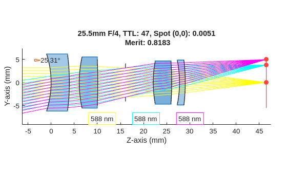
25.5mm F/4, TTL: 47, Spot (0,0): 0.0051
 Merit: 0.8183

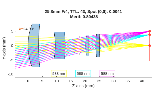
25.8mm F/4, TTL: 43, Spot (0,0): 0.0041
 Merit: 0.80438

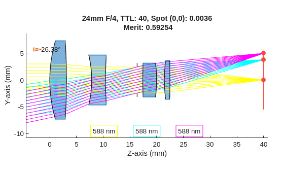
24mm F/4, TTL: 40, Spot (0,0): 0.0036
 Merit: 0.59254

Outlook

This example demonstrates how to design an optical system from the ground up, guided by specific design requirements and constraints. You use a representative set of specifications and a straightforward merit function to generate an initial, practical solution. This workflow is highly flexible, as you can further refine your design by introducing additional constraints, tuning design variables, or expanding the merit function to address more advanced objectives. For example, you can incrementally add goals for distortion, aberrations, and field curvature, along with their corresponding merit terms, to evolve your design toward real-world application.

Helper Functions

x2opsys

Convert a numeric optimization variable to an optical system object.

function opsys = x2opsys(x,design,goal)

% This function assumes a fixed configuration:
% 2 singlets + diaphragm + 2 singlets + image plane
% You can relax this, and explore different layouts, by editing
% this function.

% Unpack variables from x
dsd = x(1:design.NumSemiDiameters); % Only one SD for diaphragm
xStart = numel(dsd)+1;

xEnd = xStart+design.NumRadius-1;
cs = x(xStart:xEnd);
% Convert curvature to radius
rs = 1./cs;
xStart = xEnd+1;

xEnd = xStart+design.NumThickness-1;
ts = x(xStart:xEnd);
xStart = xEnd+1;

xEnd = xStart+design.NumGaps-1;
gs = x(xStart:xEnd);
xStart = xEnd+1;

xEnd = xStart+design.NumMaterials-1;
nds = x(xStart:xEnd);

% Snap to closest from discrete range. Because this example uses a wide range of
% available Nds, this likely does not significantly impact gradients for the optimizer
% If you are working with a smaller set, consider delaying this operation until
% after you find a candidate with continuous Nd.
nds = snapToClosest(nds,design.AvailableNds);

% Pick max semi-diameter possible, ensure its within design range
sds = max(abs(rs),design.SemidiameterRange(1));
sds = min(sds,design.SemidiameterRange(2));

% Clamp very small radii up to the min sd range
% Note: r=0 is a planar surface.
rs = max(abs(rs),sds).*sign(rs);

% Build the optical system
opsys = opticalSystem();
% Add first singlet
opsys.addRefractiveSurface(SemiDiameter=sds(1),Radius=rs(1),DistanceToNext=ts(1),Material=opticalMaterial(nds(1)))
opsys.addRefractiveSurface(SemiDiameter=sds(2),Radius=rs(2),DistanceToNext=gs(1))
% Add second singlet
opsys.addRefractiveSurface(SemiDiameter=sds(3),Radius=rs(3),DistanceToNext=ts(2),Material=opticalMaterial(nds(2)))
opsys.addRefractiveSurface(SemiDiameter=sds(4),Radius=rs(4),DistanceToNext=gs(2))

% Add diaphragm
opsys.addDiaphragm(SemiDiameter=dsd, DistanceToNext=gs(3))

% Add third singlet
opsys.addRefractiveSurface(SemiDiameter=sds(5),Radius=rs(5),DistanceToNext=ts(3),Material=opticalMaterial(nds(3)))
opsys.addRefractiveSurface(SemiDiameter=sds(6),Radius=rs(6),DistanceToNext=gs(4))
% Add fourth singlet
opsys.addRefractiveSurface(SemiDiameter=sds(7),Radius=rs(7),DistanceToNext=ts(4),Material=opticalMaterial(nds(4)))
% DistanceToNext here is the distance to the image sensor from the last
% lens surface. This is usually a fixed quantity based on the mounts and
% enclosure constraints. Make this a free variable with a small range
% if required/possible. Use 17.526 mm, the flange focal distance for a C-mount.
opsys.addRefractiveSurface(SemiDiameter=sds(8),Radius=rs(8),DistanceToNext=17.526)

% Add sensor
opsys.addImagePlane(SemiDiameter=design.SensorSemiDiag)

opsys.Wavelengths = design.Wavelength;
opsys.FieldPoints = goal.FieldPoints;

% Hit required F Number
try %#ok<TRYNC>
    p = paraxialInfo(opsys);
    updateSemiDiameters(opsys,...
        "EntryPupilRadius",p.FocalLength/2/goal.FNumber,...
        UpdateImagePlaneSize=false);
end

end

opticalMeritFunction

Compute a vector of normalized, weighted deviations between the actual and target performance metrics of an optical system design.

function merit = opticalMeritFunction(opsys,goal)

% Return merit as normalized, weighted L1 norm, (goal-act)/act*weight, as required
% by lsqnonlin

merit = [];
try
    paraInfo = paraxialInfo(opsys);
catch
    % Certain design candidates can be invalid and cause paraxialInfo to
    % fail. Pick large values, indicating poor matches.
    paraInfo.FocalLength = 1000;
end

% Focal Length
actFocalLength = paraInfo.FocalLength;
if isinf(actFocalLength)
    actFocalLength = 1000;
end
merit(end+1) = (goal.FocalLength-actFocalLength)/goal.FocalLength*goal.FocalLengthWeight;

% TTL (Total Track Length)
% Since this is a single axis design with origin at 0,0, TTL is just the
% position of the last component (image plane).
actTTL = opsys.Components(end).Position(3);
merit(end+1) = (goal.TTL-actTTL)/goal.TTL*goal.TTLWeight;

% Spot
for sInd = 1:numel(goal.FieldPoints)
    try
        spt = spot(opsys,FieldPoint=goal.FieldPoints(sInd));
        rms = spt.RMS;
        if isnan(spt.RMS)
            rms = 1;
        end
    catch
        rms = 1;
    end
    merit(end+1) = (rms-goal.SpotRMS)/goal.SpotRMS ...
        *goal.FieldPointsWeight(sInd) ...
        *goal.SpotRMSWeight;
end
end

snapToClosest

Snap a continuous Nd value to the closest discrete value in the glass library.

function snds = snapToClosest(nds,dnds)
distances = abs(nds(:) - dnds(:)');
% Find index of minimum distance for each nds value
[~,idx] = min(distances,[],2);
% Map to closest discrete values
snds = dnds(idx);
end

viewWithInfo

Visualize a system in 2-D along with its computed values and rays.

function viewWithInfo(opsys,goal)
h = view2d(opsys);
rb = traceRays(opsys);
% Color by field points
addRays(h,rb(1),Color="y")
if numel(rb) > 1
    addRays(h,rb(2),Color="c")
    addRays(h,rb(3),Color="m")
end
% Show merit info in the title
p = paraxialInfo(opsys);
h.Title = num2str(p.FocalLength,3) + "mm" ...
    + " F/"  + num2str(p.FNumber,2) ...
    + ", TTL: " + num2str(opsys.Components(end).Position(end),2) ...
    + ", Spot (0,0): "+ num2str(opsys.spot.RMS,"%1.4f") ...
    + newline ...
    + " Merit: "+ norm(opticalMeritFunction(opsys,goal));
disp(h.Title)
end