OpticalSystemViewer3D

Customize 3-D visualization of optical system

Since R2026a

Description

Add-On Required: This feature requires the Optical Design and Simulation Library for Image Processing Toolbox add-on.

An OpticalSystemViewer3D represents a 3-D visualization of an optical system. . You can customize the visualization by using the object functions of the OpticalSystemViewer3D object.

Creation

Create an OpticalSystemViewer3D object by using the view3d function to visualize an optical system in 3-D.

Properties

expand all

Optical System

`Rays` — Rays in visualization
Read-only: array of `Rays3D` objects

This property is read-only.

Rays in the visualization, represented as an array of Rays3D objects.

Label

`Title` — Title of visualization
`"Optical System"` (default) | string scalar | character vector

Title of the visualization, specified as a string scalar or character vector.

Data Types: char | string

`Labels` — Type of labels
`"none"` (default) | `"component"` | `"surface"`

Type of labels, specified as one of these options.

"component" — The visualization displays labels for only the components in the optical system.
"surface" — The visualization displays labels for each individual surface in the optical system.
"none" — The visualization does not display any labels in the optical system.

Data Types: char | string

Appearance

`ClipAngle` — Clip angle in degrees
`0` (default) | numeric scalar

Clip angle in degrees, specified as a numeric scalar. The clip angle indicates the angle at which to clip the optical components in the visualization.

`BackgroundColor` — Background color
`[0.9608 0.9608 0.9608]` (default) | RGB triplet | hexadecimal color code | `"r"` | `"g"` | `"b"` | ...

Background color, specified as an RGB triplet, a hexadecimal color code, or one of the color options listed in the table.

For a custom color, specify an RGB triplet or a hexadecimal color code.

An RGB triplet is a three-element row vector whose elements specify the intensities of the red, green, and blue components of the color. The intensities must be in the range [0,1], for example, [0.4 0.6 0.7].
A hexadecimal color code is a string scalar or character vector that starts with a hash symbol (#) followed by three or six hexadecimal digits, which can range from 0 to F. The values are not case sensitive. Therefore, the color codes "#FF8800", "#ff8800", "#F80", and "#f80" are equivalent.

Alternatively, you can specify some common colors by name. This table lists the named color options, the equivalent RGB triplets, and the hexadecimal color codes.

Color Name	Short Name	RGB Triplet	Hexadecimal Color Code	Appearance
`"red"`	`"r"`	`[1 0 0]`	`"#FF0000"`
`"green"`	`"g"`	`[0 1 0]`	`"#00FF00"`
`"blue"`	`"b"`	`[0 0 1]`	`"#0000FF"`
`"cyan"`	`"c"`	`[0 1 1]`	`"#00FFFF"`
`"magenta"`	`"m"`	`[1 0 1]`	`"#FF00FF"`
`"yellow"`	`"y"`	`[1 1 0]`	`"#FFFF00"`
`"black"`	`"k"`	`[0 0 0]`	`"#000000"`
`"white"`	`"w"`	`[1 1 1]`	`"#FFFFFF"`
`"none"`	Not applicable	Not applicable	Not applicable	No color

`BackgroundGradient` — Background gradient display
`"on"` (default) | on/off logical value

Background gradient display, specified as "on" or "off", matlab.lang.OnOffSwitchState.on or matlab.lang.OnOffSwitchState.off, or as numeric or logical 1 (true) or 0 (false). A value of "on" is equivalent to a logical on or true, and "off" is equivalent to a logical off or false. Thus, you can use the value of this property as a logical value. The value is stored as an on/off logical value of type matlab.lang.OnOffSwitchState.

If you specify BackgroundGradient as "on", matlab.lang.OnOffSwitchState.on, or as a numeric or logical 1 (true), the function displays a background gradient in the visualization.

`GradientColor` — Gradient color
`[0.9020 0.9020 0.9020]` (default) | RGB triplet | hexadecimal color code | `"r"` | `"g"` | `"b"` | ...

Gradient color, specified as an RGB triplet, a hexadecimal color code, or one of the color options listed in the table.

For a custom color, specify an RGB triplet or a hexadecimal color code.

An RGB triplet is a three-element row vector whose elements specify the intensities of the red, green, and blue components of the color. The intensities must be in the range [0,1], for example, [0.4 0.6 0.7].
A hexadecimal color code is a string scalar or character vector that starts with a hash symbol (#) followed by three or six hexadecimal digits, which can range from 0 to F. The values are not case sensitive. Therefore, the color codes "#FF8800", "#ff8800", "#F80", and "#f80" are equivalent.

Alternatively, you can specify some common colors by name. This table lists the named color options, the equivalent RGB triplets, and the hexadecimal color codes.

Color Name	Short Name	RGB Triplet	Hexadecimal Color Code	Appearance
`"red"`	`"r"`	`[1 0 0]`	`"#FF0000"`
`"green"`	`"g"`	`[0 1 0]`	`"#00FF00"`
`"blue"`	`"b"`	`[0 0 1]`	`"#0000FF"`
`"cyan"`	`"c"`	`[0 1 1]`	`"#00FFFF"`
`"magenta"`	`"m"`	`[1 0 1]`	`"#FF00FF"`
`"yellow"`	`"y"`	`[1 1 0]`	`"#FFFF00"`
`"black"`	`"k"`	`[0 0 0]`	`"#000000"`
`"white"`	`"w"`	`[1 1 1]`	`"#FFFFFF"`
`"none"`	Not applicable	Not applicable	Not applicable	No color

Position

`OuterPosition` — Chart size and location, including margins
4-element numeric vector

Chart size and location, including the margins, specified as a 4-element numeric vector of the form [left bottom width height]. The values are in the units specified by the Units property.

left — Distance from the left edge of the parent container to the outer-left margin of the chart.
bottom — Distance from the bottom edge of the parent container to the outer-bottom margin of the chart.
width — Width of chart, including the margins.
height — Height of chart, including the margins.

`InnerPosition` — Chart size and location, excluding margins
4-element numeric vector

Chart size and location, excluding the margins, specified as a 4-element numeric vector of the form [left bottom width height]. The values are in the units specified by the Units property.

left — Distance from the left edge of the parent container to the inner-left edge of the chart, past the margins.
bottom — Distance from the bottom edge of the parent container to the inner-bottom edge of the chart, past the margins.
width — Width of the chart, excluding the margins.
height — Height of the chart, excluding the margins.

`Position` — Chart size and location, excluding margins
4-element numeric vector

Chart size and location, excluding the margins, specified as a 4-element numeric vector of the form [left bottom width height]. This property is equivalent to the InnerPosition property.

`PositionConstraint` — Position to hold constant
`"outerposition"` (default) | `"innerposition"`

Position property to hold constant when adding, removing, or changing decorations, specified as one of these values.

"outerposition" — The OuterPosition property remains constant when you add, remove, or change decorations such as a title or an axis label. If any changes require positional adjustments, MATLAB^® adjusts the InnerPosition property.
"innerposition" — The InnerPosition property remains constant when you add, remove, or change decorations such as a title or an axis label. If any changes require positional adjustments, MATLAB adjusts the OuterPosition property.

`Units` — Position units
`"normalized"` (default) | `"inches"` | `"centimeters"` | `"characters"` | `"points"` | `"pixels"`

Position units, specified as one of these values.

`Units`	Description
`"normalized"`	Normalized with respect to the parent container. The lower-left corner of the container maps to `(0,0)`, and the upper-right corner maps to `(1,1)`.
`"inches"`	Inches.
`"centimeters"`	Centimeters.
`"characters"`	Based on the default font of the graphics root object. Character width is the width of the letter `x`. Character height is the distance between the baselines of two lines of text.
`"points"`	Typography points. One point equals 1/72 inch.
`"pixels"`	Pixels. On Windows^® and Macintosh systems, the size of a pixel is 1/96 inch. This size is independent of your system resolution. On Linux^® systems, the size of a pixel is determined by your system resolution.

To change the position of the chart in specific units, set the Units property before specifying the Position property. If you specify the Units and Position properties in a single command using name-value arguments, be sure to specify Units before Position.

`Layout` — Layout options
empty `LayoutOptions` array (default) | `GridLayoutOptions` object

Layout options, specified as a GridLayoutOptions object. This property specifies layout options when the parent container is a GridLayout object. You can place the chart in the desired row and column of the parent grid by setting the Row and Column properties on the GridLayoutOptions object.

For example, this code places the chart object osv into the third row and fifth column of a grid layout.

osv.Layout.Row = 3;
osv.Layout.Column = 5;

Visibility

`Visible` — State of visibility
`"on"` (default) | on/off logical value

State of visibility, specified as "on" or "off", matlab.lang.OnOffSwitchState.on or matlab.lang.OnOffSwitchState.off, or as numeric or logical 1 (true) or 0 (false). A value of "on" is equivalent to a logical on or true, and "off" is equivalent to a logical off or false. Thus, you can use the value of this property as a logical value. The value is stored as an on/off logical value of type matlab.lang.OnOffSwitchState.

If you specify Visible as "on", matlab.lang.OnOffSwitchState.on, or as a numeric or logical 1 (true), the function displays the chart. Otherwise, the function hides the chart without deleting it. You still can access the properties of the chart when it is not visible.

Parent/Child

`Parent` — Parent UI container
`Figure` object | `Panel` object | `Tab` object | `GridLayout` object

Parent UI container, specified as a Figure, Panel, Tab, or GridLayout object. By default, the function creates a new Figure object. You can create these UI containers using their respective creation functions.

Figure object — uifigure
Panel object — uipanel
Tab object — uitab
GridLayout object — uigridlayout

`HandleVisibility` — Visibility of chart object handle
`"on"` (default) | `"off"` | `"callback"`

Visibility of the chart object handle, specified as "on", "off", or "callback". This property determines the visibility of the chart object handle in the list of children of its parent object..

"on" — Chart object handle is always visible.
"off" — Chart object handle is invisible at all times. You can use this option to prevent unintended changes to the chart by another function by temporarily hiding the handle. To do so, for the duration of the execution of that function, set HandleVisibility to "off".
"callback" — Chart object handle is visible from within callbacks or functions invoked by callbacks, but not from within functions invoked from the command line. This option blocks access to the object in the Command Window, but it allows callback functions to access the object.

Object Functions

`addRays`	Add traced rays to visualization of optical system
`removeRays`	Remove traced rays from visualization of optical system
`explode`	Explode components in 3-D optical system visualization radially outward
`unexplode`	Restore original component locations in 3-D optical system visualization after explosion
`showComponents`	Show selected components in 3-D optical system visualization

Examples

collapse all

Visualize Optical System in 3-D

This example uses:

Optical Design and Simulation Library for Image Processing Toolbox Optical Design and Simulation Library for Image Processing Toolbox

Open Live Script

Create a simple optical system.

opsys = opticalSystem;
addRefractiveSurface(opsys,Radius=9,Material=[1.74 25.4],DistanceToNext=3) 
addRefractiveSurface(opsys,Radius=-9,DistanceToNext=10)
addImagePlane(opsys)

Visualize the optical system in 3-D.

osv3d = view3d(opsys,Title="Convex Lens")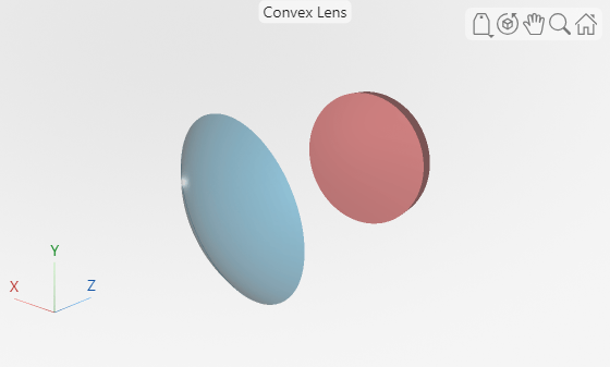

osv3d = 
  OpticalSystemViewer3D with properties:

              Title: [0×0 string]
             Labels: "none"
          ClipAngle: 0
               Rays: [0×0 optics.ui.Rays3D]
    BackgroundColor: [0.9608 0.9608 0.9608]
      GradientColor: [0.9020 0.9020 0.9020]
             Parent: [1×1 Figure]

  Show all properties

Trace rays in the optical system to add to the visualization. Observe that rays contains three ray bundles.

rays = traceRays(opsys)

rays=1×3 RayBundle array with properties:
    1×1 RayBundle    1×1 RayBundle    1×1 RayBundle

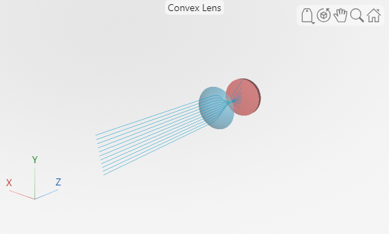
You can add only one ray bundle to a 3-D visualization. Add one of the ray bundles from the traced rays to the visualization.

addRays(osv3d,rays(1))

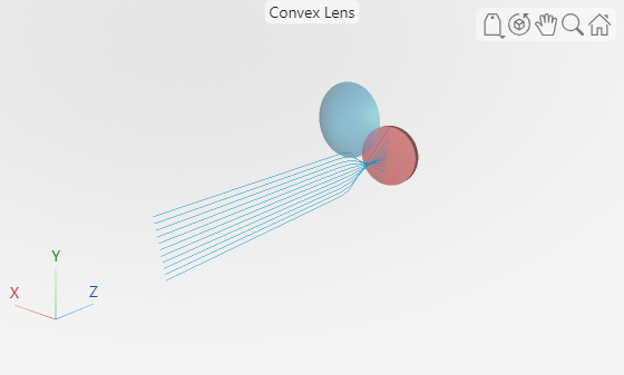
Explode the visualization. The explosion moves each component in the optical system visualization radially outward to enable you to better visualize the internal structure of the optical system.

explode(osv3d)

Restore the visualization to its state before the explosion.

unexplode(osv3d)

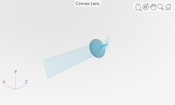
Show only the lens element, which is the first optical component, in the visualization.

showComponents(osv3d,1)

Remove the rays from the visualization.

removeRays(osv3d)

Add component labels to the visualization.

osv3d.Labels = "component";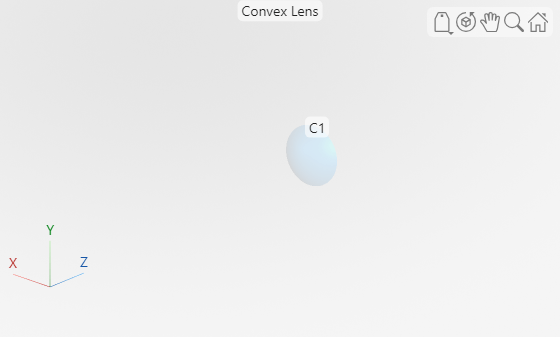

Version History

Introduced in R2026a

OpticalSystemViewer3D

Description

Creation

Properties

Optical System

Rays — Rays in visualization Read-only: array of Rays3D objects

Label

Title — Title of visualization "Optical System" (default) | string scalar | character vector

Labels — Type of labels "none" (default) | "component" | "surface"

Appearance

ClipAngle — Clip angle in degrees 0 (default) | numeric scalar

BackgroundColor — Background color [0.9608 0.9608 0.9608] (default) | RGB triplet | hexadecimal color code | "r" | "g" | "b" | ...

BackgroundGradient — Background gradient display "on" (default) | on/off logical value

GradientColor — Gradient color [0.9020 0.9020 0.9020] (default) | RGB triplet | hexadecimal color code | "r" | "g" | "b" | ...

Position

OuterPosition — Chart size and location, including margins 4-element numeric vector

InnerPosition — Chart size and location, excluding margins 4-element numeric vector

Position — Chart size and location, excluding margins 4-element numeric vector

PositionConstraint — Position to hold constant "outerposition" (default) | "innerposition"

Units — Position units "normalized" (default) | "inches" | "centimeters" | "characters" | "points" | "pixels"

Layout — Layout options empty LayoutOptions array (default) | GridLayoutOptions object