OpticalSystemViewer2D
Description
Add-On Required: This feature requires the Optical Design and Simulation Library for Image Processing Toolbox add-on.
An OpticalSystemViewer2D represents a 2-D visualization of an
optical system. . You can customize the visualization by using the object functions of the
OpticalSystemViewer2D object.
Creation
Create an OpticalSystemViewer2D object by using the view2d function
to visualize an optical system in 2-D.
Properties
Optical System
Rays in the visualization, specified as an array of Rays2D
objects.
Field points in visualization, specified as an array of Rays2D
objects, specified as "on", "off",
matlab.lang.OnOffSwitchState.on or
matlab.lang.OnOffSwitchState.off, or as numeric or logical
1 (true) or 0
(false). A value of "on" is equivalent to a
logical on or true, and "off" is equivalent to a
logical off or false. Thus, you can use the value of this property
as a logical value. The value is stored as an on/off logical value of type matlab.lang.OnOffSwitchState.
By default, the object displays the field points of the optical system
opsys in the visualization. If you specify
FieldPoints as "off",
matlab.lang.OnOffSwitchState.off, or as a numeric or logical
0 (true), the object does not display the
field points in the visualization.
For more information about field points, see Create Field Points.
Paraxial information display, specified as "on" or
"off", matlab.lang.OnOffSwitchState.on or
matlab.lang.OnOffSwitchState.off, or as numeric or logical
1 (true) or 0
(false). A value of "on" is equivalent to a
logical on or true, and "off" is equivalent to a
logical off or false. Thus, you can use the value of this property
as a logical value. The value is stored as an on/off logical value of type matlab.lang.OnOffSwitchState.
If you specify ParaxialInfo as "on",
matlab.lang.OnOffSwitchState.on, or as a numeric or logical
1 (true), the object displays the paraxial
information in the visualization.
Data Types: single | double | int8 | int16 | int32 | int64 | uint8 | uint16 | uint32 | uint64 | logical
Label
Title of the visualization, represented as a string scalar.
Data Types: string
Type of labels, specified as one of these options.
"component"— The visualization displays labels for only the components in the optical system."surface"— The visualization displays labels for each individual surface in the optical system."none"— The visualization does not display any labels in the optical system."both"— The visualization displays labels for each individual surface and each component in the optical system.
Data Types: char | string
Appearance
Z-axis limits, specified as a 2-element numeric vector of the
form [zmin
zmax]. zmin and
zmax are the lower and upper limits of the
z-axis, respectively. The default value is adjusted to fit the
optical system.
Data Types: single | double | int8 | int16 | int32 | int64 | uint8 | uint16 | uint32 | uint64
Y-axis limits, specified as a 2-element numeric vector of the
form [ymin
ymax]. ymin and
ymax are the lower and upper limits of the
y-axis, respectively. The default value is adjusted to fit the
optical system.
Data Types: single | double | int8 | int16 | int32 | int64 | uint8 | uint16 | uint32 | uint64
Z-axis limits, specified as a 2-element numeric vector of the
form [zmin
zmax]. zmin and
zmax are the lower and upper limits of the
z-axis, respectively. The default value is adjusted to fit the
optical system.
Data Types: single | double | int8 | int16 | int32 | int64 | uint8 | uint16 | uint32 | uint64
Selection mode for the Z-axis limit, specified as one of these values:
"auto"— Enable automatic limit selection, which is based on the total span of the plotted data."manual"— Manually specify the axis limits. To specify the axis limits, set theYLimorZLimproperty.
Data Types: single | double | int8 | int16 | int32 | int64 | uint8 | uint16 | uint32 | uint64
Selection mode for the Y-axis limit, specified as one of these values:
"auto"— Enable automatic limit selection, which is based on the total span of the plotted data."manual"— Manually specify the axis limits. To specify the axis limits, set theYLimorZLimproperty.
Data Types: single | double | int8 | int16 | int32 | int64 | uint8 | uint16 | uint32 | uint64
Position
Chart size and location, including the margins, specified as a 4-element numeric
vector of the form [left bottom width height]. The values are in
the units specified by the Units property.
left— Distance from the left edge of the parent container to the outer-left margin of the chart.bottom— Distance from the bottom edge of the parent container to the outer-bottom margin of the chart.width— Width of chart, including the margins.height— Height of chart, including the margins.
Chart size and location, excluding the margins, specified as a 4-element numeric
vector of the form [left bottom width height]. The values are in
the units specified by the Units property.
left— Distance from the left edge of the parent container to the inner-left edge of the chart, past the margins.bottom— Distance from the bottom edge of the parent container to the inner-bottom edge of the chart, past the margins.width— Width of the chart, excluding the margins.height— Height of the chart, excluding the margins.
Chart size and location, excluding the margins, specified as a 4-element numeric
vector of the form [left bottom width height]. This property is
equivalent to the InnerPosition property.
Position property to hold constant when adding, removing, or changing decorations, specified as one of these values.
"outerposition"— TheOuterPositionproperty remains constant when you add, remove, or change decorations such as a title or an axis label. If any changes require positional adjustments, MATLAB® adjusts theInnerPositionproperty."innerposition"— TheInnerPositionproperty remains constant when you add, remove, or change decorations such as a title or an axis label. If any changes require positional adjustments, MATLAB adjusts theOuterPositionproperty.
Position units, specified as one of these values.
Units | Description |
|---|---|
"normalized" | Normalized with respect to the parent container. The lower-left corner
of the container maps to (0,0), and the upper-right
corner maps to (1,1). |
"inches" | Inches. |
"centimeters" | Centimeters. |
"characters" | Based on the default font of the graphics root object.
|
"points" | Typography points. One point equals 1/72 inch. |
"pixels" | Pixels. On Windows® and Macintosh systems, the size of a pixel is 1/96 inch. This size is independent of your system resolution. On Linux® systems, the size of a pixel is determined by your system resolution. |
To change the position of the chart in specific units, set the
Units property before specifying the
Position property. If you specify the
Units and Position properties in a single
command using name-value arguments, be sure to specify Units
before Position.
Layout options, specified as a GridLayoutOptions object. This
property specifies layout options when the parent container is a
GridLayout object. You can place the chart in the desired row and
column of the parent grid by setting the Row and
Column properties on the GridLayoutOptions
object.
For example, this code places the chart object osv into the
third row and fifth column of a grid
layout.
osv.Layout.Row = 3; osv.Layout.Column = 5;
Visibility
State of visibility, specified as "on" or
"off", matlab.lang.OnOffSwitchState.on or
matlab.lang.OnOffSwitchState.off, or as numeric or logical
1 (true) or 0
(false). A value of "on" is equivalent to a
logical on or true, and "off" is equivalent to a
logical off or false. Thus, you can use the value of this property
as a logical value. The value is stored as an on/off logical value of type matlab.lang.OnOffSwitchState.
If you specify Visible as "on",
matlab.lang.OnOffSwitchState.on, or as a numeric or logical
1 (true), the object displays the chart.
Otherwise, the object hides the chart without deleting it. You still can access the
properties of the chart when it is not visible.
Parent/Child
Parent UI container, specified as a Figure,
Panel, Tab, or GridLayout
object. By default, the object creates a new Figure object. You can
create these UI containers using their respective creation functions.
Figureobject —uifigurePanelobject —uipanelTabobject —uitabGridLayoutobject —uigridlayout
Visibility of the chart object handle, specified as "on",
"off", or "callback". This property determines
the visibility of the chart object handle in the list of children of its parent object..
"on"— Chart object handle is always visible."off"— Chart object handle is invisible at all times. You can use this option to prevent unintended changes to the chart by another function by temporarily hiding the handle. To do so, for the duration of the execution of that function, setHandleVisibilityto"off"."callback"— Chart object handle is visible from within callbacks or functions invoked by callbacks, but not from within functions invoked from the command line. This option blocks access to the object in the Command Window, but it allows callback functions to access the object.
Object Functions
addRays | Add traced rays to visualization of optical system |
removeRays | Remove traced rays from visualization of optical system |
Examples
Create a simple optical system.
opsys = opticalSystem; addRefractiveSurface(opsys,Radius=9,Material=[1.74 25.4],DistanceToNext=3) addRefractiveSurface(opsys,Radius=-9,DistanceToNext=10) addImagePlane(opsys) focus(opsys);
Visualize the optical system in 2-D.
osv2d = view2d(opsys,Title="Convex Lens")
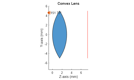
osv2d =
OpticalSystemViewer2D with properties:
Title: "Convex Lens"
OpticalSystem: [1×1 opticalSystem]
Labels: "none"
FieldPoints: "on"
Rays: [0×0 optics.ui.Rays2D]
Parent: [1×1 Figure]
Show all properties
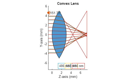
Trace rays in the optical system to add to the visualization. Observe that rays contains three ray bundles.
rays = traceRays(opsys)
rays=1×3 RayBundle array with properties:
FieldPoint
Wavelength
Sampling
RayData
Add the rays to the visualization. Each ray bundle is represented by a different color in the visualization.
addRays(osv2d,rays)

Remove the third ray bundle in the visualization.
removeRays(osv2d,3)

Add component labels to the visualization. The lens and image plane components are labeled as C1 and C2 in the visualization.
osv2d.Labels = "component";
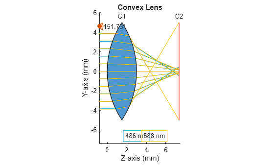
Version History
Introduced in R2026a
See Also
MATLAB Command
You clicked a link that corresponds to this MATLAB command:
Run the command by entering it in the MATLAB Command Window. Web browsers do not support MATLAB commands.
选择网站
选择网站以获取翻译的可用内容,以及查看当地活动和优惠。根据您的位置,我们建议您选择:。
您也可以从以下列表中选择网站:
如何获得最佳网站性能
选择中国网站(中文或英文)以获得最佳网站性能。其他 MathWorks 国家/地区网站并未针对您所在位置的访问进行优化。
美洲
- América Latina (Español)
- Canada (English)
- United States (English)
欧洲
- Belgium (English)
- Denmark (English)
- Deutschland (Deutsch)
- España (Español)
- Finland (English)
- France (Français)
- Ireland (English)
- Italia (Italiano)
- Luxembourg (English)
- Netherlands (English)
- Norway (English)
- Österreich (Deutsch)
- Portugal (English)
- Sweden (English)
- Switzerland
- United Kingdom (English)