基于问题求解有约束非线性问题：

打开实时脚本

典型优化问题

此示例说明如何使用基于问题的方法来求解有约束非线性优化问题。该示例展示了典型的工作流：创建目标函数、创建约束、求解问题和检查结果。

注意：

如果目标函数或非线性约束不是由初等函数组成，则必须使用 fcn2optimexpr 将非线性函数转换为优化表达式。请参阅此示例的最后一部分，使用 fcn2optimexpr 的替代表示，或将非线性函数转换为优化表达式。

要了解如何通过基于求解器的方法处理此问题，请参阅使用优化实时编辑器任务或求解器的有约束非线性问题。

问题表示：罗森布罗克函数

假设问题是最小化 1 加上罗森布罗克函数的对数

$f (x) = \log (1 + 100 {(x_{2} - x_{1}^{2})}^{2} + (1 - x_{1})^{2}),$

单位圆盘是以原点为圆心、半径为 1 的圆。也就是说，基于数据集 $x_{1}^{2} + x_{2}^{2} \leq 1$ ，求使函数 $f (x)$ 最小的 $x$ 。此问题是非线性约束下的非线性函数最小化问题。

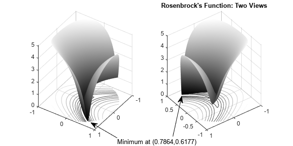
罗森布罗克函数是优化中的标准测试函数。它在点 [1,1] 处达到唯一最小值 0，因此 $f (x)$ 在同一点处达到相同的最小值。对于某些算法来说，求最小值是一个挑战，因为函数在深度弯曲的波谷中有一个低浅最小值。此问题的解不在 [1,1] 点处，因为该点不满足约束。

以下图窗显示了单位圆盘中函数 $f (x)$ 的两个视图。等高线位于曲面图下方。

rosenbrock = @(x)log(1 + 100*(x(:,2) - x(:,1).^2).^2 + (1 - x(:,1)).^2); % Vectorized function

figure1 = figure('Position',[1 200 600 300]);
colormap('gray');
axis square;
R = 0:.002:1;
TH = 2*pi*(0:.002:1); 
X = R'*cos(TH);
Y = R'*sin(TH); 
Z = rosenbrock([X(:),Y(:)]); % Z = f(x)
Z = reshape(Z,size(X));

% Create subplot
subplot1 = subplot(1,2,1,'Parent',figure1);
view([124 34]);
grid('on');
hold on;

% Create surface
surf(X,Y,Z,'Parent',subplot1,'LineStyle','none');

% Create contour
contour(X,Y,Z,'Parent',subplot1);

% Create subplot
subplot2 = subplot(1,2,2,'Parent',figure1);
view([234 34]);
grid('on');
hold on

% Create surface
surf(X,Y,Z,'Parent',subplot2,'LineStyle','none');

% Create contour
contour(X,Y,Z,'Parent',subplot2);

% Create textarrow
annotation(figure1,'textarrow',[0.4 0.31],...
    [0.055 0.16],...
    'String',{'Minimum at (0.7864,0.6177)'});

% Create arrow
annotation(figure1,'arrow',[0.59 0.62],...
    [0.065 0.34]);

title("Rosenbrock's Function: Two Views")

hold off

rosenbrock 函数句柄同时在任意数量的二维点处计算函数 $f (x)$ 。这种向量化可加快函数的绘图速度，在用于加快在多个点的函数计算速度的其他环境中很有用。

函数 $f (x)$ 称为目标函数。目标函数是您要进行最小化的函数。不等式 $x_{1}^{2} + x_{2}^{2} \leq 1$ 称为约束。约束限制求解器用于搜索最小值的 $x$ 集。您可以使用任意数量的约束，约束可以是不等式，也可以是方程。

使用优化变量定义问题

基于问题的优化方法使用优化变量来定义目标和约束。使用这些变量创建表达式有两种方法：

对于多项式或三角函数等初等函数，直接使用变量编写表达式。
对于其他类型的函数，使用 fcn2optimexpr 将函数转换为优化表达式。请参阅此示例末尾的使用 fcn2optimexpr 的替代表示。

对于此问题，目标函数和非线性约束均为初等函数，因此，您可以直接用优化变量来编写表达式。创建名为 'x' 的二维优化变量。

x = optimvar('x',1,2);

使用优化变量的表达式创建目标函数。

obj = log(1 + 100*(x(2) - x(1)^2)^2 + (1 - x(1))^2);

以 obj 为目标函数，创建名为 prob 的优化问题。

prob = optimproblem('Objective',obj);

创建非线性约束作为优化变量的多项式。

nlcons = x(1)^2 + x(2)^2 <= 1;

在问题中包含非线性约束。

prob.Constraints.circlecons = nlcons;

检查此问题。

show(prob)

  OptimizationProblem : 

	Solve for:
       x

	minimize :
       log(((1 + (100 .* (x(2) - x(1).^2).^2)) + (1 - x(1)).^2))


	subject to circlecons:
       (x(1).^2 + x(2).^2) <= 1

求解问题

要求解优化问题，请调用 solve。此问题需要一个初始点，它是给出优化变量初始值的结构体。创建初始点结构体 x0， $x$ 值为 [0 0]。

x0.x = [0 0];
[sol,fval,exitflag,output] = solve(prob,x0)

Solving problem using fmincon.

Local minimum found that satisfies the constraints.

Optimization completed because the objective function is non-decreasing in 
feasible directions, to within the value of the optimality tolerance,
and constraints are satisfied to within the value of the constraint tolerance.

sol = struct with fields:
    x: [0.7864 0.6177]

fval = 0.0447

exitflag = 
    OptimalSolution

output = struct with fields:
              iterations: 23
               funcCount: 44
         constrviolation: 0
                stepsize: 7.7862e-09
               algorithm: 'interior-point'
           firstorderopt: 8.0000e-08
            cgiterations: 8
                 message: 'Local minimum found that satisfies the constraints....'
            bestfeasible: [1x1 struct]
     objectivederivative: "reverse-AD"
    constraintderivative: "closed-form"
                  solver: 'fmincon'

检查解

该解显示 exitflag = OptimalSolution。此退出标志表示该解是局部最优值。有关尝试求更优解的信息，请参阅求解成功后。

退出消息表明解满足约束。您可以从几个方面检查该解是否确实可行。

检查在 output 结构体的 constrviolation 字段中报告的不可行性。

infeas = output.constrviolation

infeas = 0

不可行性为 0 表明该解可行。

计算在解处的不可行性。

infeas = infeasibility(nlcons,sol)

infeas = 0

同样，不可行性为 0 表明该解可行。

计算 x 的范数，以确保它小于或等于 1。

nx = norm(sol.x)

nx = 1.0000

output 结构体提供有关求解过程的详细信息，例如迭代次数（23 次）、求解器 (fmincon) 和函数计算次数（44 次）。有关这些统计量的详细信息，请参阅容差和停止条件。

使用 `fcn2optimexpr` 的替代表示

对于更复杂的表达式，请为目标函数或约束函数编写函数文件，并使用 fcn2optimexpr 将其转换为优化表达式。例如，非线性约束函数的基础代码位于在 disk.m 文件中：

type disk

function radsqr = disk(x) 

radsqr = x(1)^2 + x(2)^2;

将此函数文件转换为优化表达式。

radsqexpr = fcn2optimexpr(@disk,x);

此外，您还可以将在绘图例程开始时定义的 rosenbrock 函数句柄转换为优化表达式。

rosenexpr = fcn2optimexpr(rosenbrock,x);

使用这些转换后的优化表达式创建优化问题。

convprob = optimproblem('Objective',rosenexpr,'Constraints',radsqexpr <= 1);

查看新问题。

show(convprob)

  OptimizationProblem : 

	Solve for:
       x

	minimize :
       log(((1 + (100 .* (x(2) - x(1).^2).^2)) + (1 - x(1)).^2))


	subject to :
       (x(1).^2 + x(2).^2) <= 1

求解新问题。解与以前的解基本相同。

[sol,fval,exitflag,output] = solve(convprob,x0)

Solving problem using fmincon.

Local minimum found that satisfies the constraints.

Optimization completed because the objective function is non-decreasing in 
feasible directions, to within the value of the optimality tolerance,
and constraints are satisfied to within the value of the constraint tolerance.

sol = struct with fields:
    x: [0.7864 0.6177]

fval = 0.0447

exitflag = 
    OptimalSolution

output = struct with fields:
              iterations: 23
               funcCount: 44
         constrviolation: 0
                stepsize: 7.7862e-09
               algorithm: 'interior-point'
           firstorderopt: 8.0000e-08
            cgiterations: 8
                 message: 'Local minimum found that satisfies the constraints....'
            bestfeasible: [1x1 struct]
     objectivederivative: "reverse-AD"
    constraintderivative: "closed-form"
                  solver: 'fmincon'

有关支持的函数列表，请参阅Supported Operations for Optimization Variables and Expressions。

基于问题求解有约束非线性问题：

典型优化问题

问题表示：罗森布罗克函数

使用优化变量定义问题

求解问题

检查解

使用 fcn2optimexpr 的替代表示

相关主题

WeChat

使用 `fcn2optimexpr` 的替代表示