主要内容

meanfreq

R2026b

Mean frequency

Description

Time-Domain Inputs

fMean = meanfreq(x) estimates the mean normalized frequency, fMean, of the power spectrum of a time-domain signal, x.

  • Specify x as a vector, matrix, or a MATLAB® timetable (since R2026b). If x is a matrix or a timetable, then the function computes the mean frequency of each column or variable independently.

  • To compute the power spectrum, meanfreq uses the periodogram function with a rectangular window and number of DFT points equal to the length of x.

example

fMean = meanfreq(x,Fs) estimates the mean frequency of x (vector or matrix) with a sample rate Fs.

example

fMean = meanfreq(x,Ts) estimates the mean frequency of x (vector or matrix) with a sample time Ts. (since R2026b)

fMean = meanfreq(x,t,Domain="time") estimates the mean frequency of x (vector or matrix) with time instances t. (since R2026b)

Note

Specify Domain="time" to distinguish time-domain inputs (x,t) from frequency-domain inputs (pxx,f).

Frequency-Domain Inputs

fMean = meanfreq(pxx,f) returns the mean frequency of a power spectral density (PSD) estimate, pxx. The frequencies, f, correspond to the estimates in pxx.

example

fMean = meanfreq(sxx,f,rbw) returns the mean frequency of a power spectrum estimate, sxx, with resolution bandwidth rbw. The frequencies, f, correspond to the estimates in sxx.

Additional Options

fMean = meanfreq(___,freqRange) specifies the frequency interval freqRange over which to compute the mean frequency.

  • This syntax can include any combination of input arguments from previous syntaxes, as long as you specify freqRange before the Domain name-value argument.

  • If you specify the second input as empty and x is not a timetable, then the function assumes normalized frequencies.

example

fMean = meanfreq(___,Domain=sigDomain) specifies the signal domain of the input. (since R2026b)

[fMean,bandPow] = meanfreq(___) also returns the band power of the spectrum, bandPow. If you specify freqRange, then bandPow contains the band power within freqRange.

example

meanfreq(___) with no output arguments plots the PSD or power spectrum and annotates the mean frequency.

example

Examples

collapse all

Generate 1024 samples of a chirp sampled at 1024 kHz. The chirp has an initial frequency of 50 kHz and reaches 100 kHz at the end of the sampling. Add white Gaussian noise such that the signal-to-noise ratio is 40 dB.

nSamp = 1024;
Fs = 1024e3;
SNR = 40;

t = (0:nSamp-1)'/Fs;
x0 = chirp(t,50e3,nSamp/Fs,100e3);

x1 = x0 + randn(size(x0))*std(x0)/db2mag(SNR);

Estimate the mean frequency of the chirp. Plot the power spectral density (PSD) and annotate the mean frequency.

meanfreq(x1,Fs);
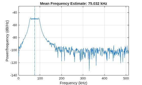
Figure contains an axes object. The axes object with title Mean Frequency Estimate: 75.032 kHz, xlabel Frequency (kHz), ylabel Power/frequency (dB/Hz) contains 2 objects of type line.

Generate another chirp. Specify an initial frequency of 200 kHz, a final frequency of 300 kHz, and an amplitude that is twice that of the first signal. Add white Gaussian noise.

x2 = 2*chirp(t,200e3,nSamp/Fs,300e3);
x2 = x2 + randn(size(x2))*std(x2)/db2mag(SNR);

Concatenate the chirps to produce a two-channel signal. Estimate the mean frequency of each channel.

y = meanfreq([x1 x2],Fs)
y = 1×2
105 ×

    0.7503    2.4999

Plot the PSDs of the two channels and annotate their mean frequencies.

meanfreq([x1 x2],Fs);
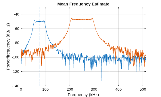
Figure contains an axes object. The axes object with title Mean Frequency Estimate, xlabel Frequency (kHz), ylabel Power/frequency (dB/Hz) contains 4 objects of type line.

Add the two channels to form a new signal. Plot the PSD and annotate the mean frequency.

meanfreq(x1+x2,Fs);
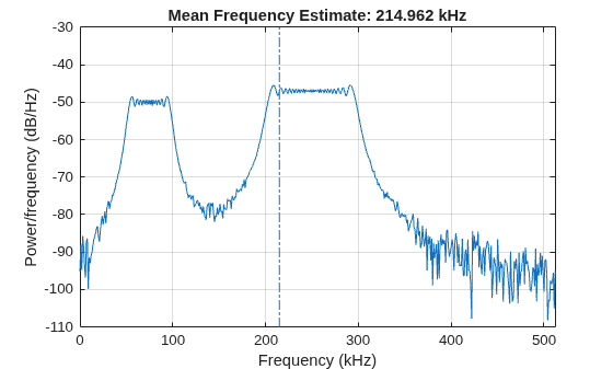
Figure contains an axes object. The axes object with title Mean Frequency Estimate: 214.962 kHz, xlabel Frequency (kHz), ylabel Power/frequency (dB/Hz) contains 2 objects of type line.

Generate 1024 samples of a 100.123 kHz sinusoid sampled at 1024 kHz. Add white Gaussian noise such that the signal-to-noise ratio is 40 dB.

nSamp = 1024;
Fs = 1024e3;
SNR = 40;

t = (0:nSamp-1)'/Fs;
x0 = sin(2*pi*t*100.123e3);

x1 = x0 + randn(size(x0))*std(x0)/db2mag(SNR);

Use the periodogram function to compute the power spectral density (PSD) of the signal. Specify a Kaiser window with the same length as the signal and a shape factor of 38. Estimate the mean frequency of the signal and annotate it on a plot of the PSD.

[Pxx,f] = periodogram(x1,kaiser(nSamp,38),[],Fs);

meanfreq(Pxx,f);
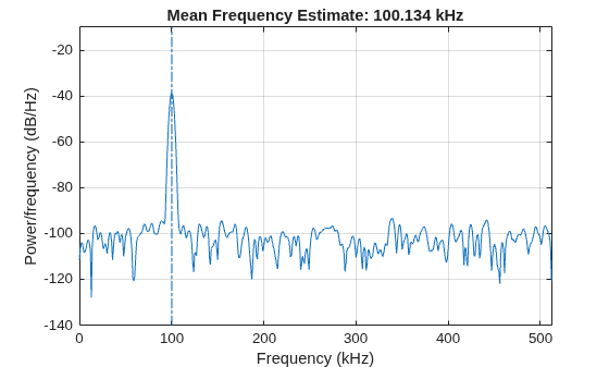
Figure contains an axes object. The axes object with title Mean Frequency Estimate: 100.134 kHz, xlabel Frequency (kHz), ylabel Power/frequency (dB/Hz) contains 2 objects of type line.

Generate another sinusoid, this one with a frequency of 257.321 kHz and an amplitude that is twice that of the first sinusoid. Add white noise.

x2 = 2*sin(2*pi*t*257.321e3);
x2 = x2 + randn(size(x2))*std(x2)/db2mag(SNR);

Concatenate the sinusoids to produce a two-channel signal. Estimate the PSD of each channel and use the result to determine the mean frequency.

[Pyy,f] = periodogram([x1 x2],kaiser(nSamp,38),[],Fs);

y = meanfreq(Pyy,f)
y = 1×2
105 ×

    1.0013    2.5732

Annotate the mean frequencies of the two channels on a plot of the PSDs.

meanfreq(Pyy,f);
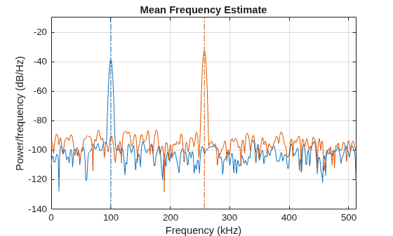
Figure contains an axes object. The axes object with title Mean Frequency Estimate, xlabel Frequency (kHz), ylabel Power/frequency (dB/Hz) contains 4 objects of type line.

Add the two channels to form a new signal. Estimate the PSD and annotate the mean frequency.

[Pzz,f] = periodogram(x1+x2,kaiser(nSamp,38),[],Fs);

meanfreq(Pzz,f);
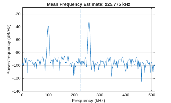
Figure contains an axes object. The axes object with title Mean Frequency Estimate: 225.775 kHz, xlabel Frequency (kHz), ylabel Power/frequency (dB/Hz) contains 2 objects of type line.

Generate a signal whose PSD resembles the frequency response of an 88th-order bandpass FIR filter with normalized cutoff frequencies 0.25π rad/sample and 0.45π rad/sample.

d = fir1(88,[0.25 0.45]);

Compute the mean frequency of the signal between 0.3π rad/sample and 0.6π rad/sample. Plot the PSD and annotate the mean frequency and measurement interval.

meanfreq(d,[],[0.3 0.6]*pi);
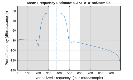
Figure contains an axes object. The axes object with title Mean Frequency Estimate: 0 . 373 times pi rad/sample, xlabel Normalized Frequency ( times pi mrad/sample), ylabel Power/frequency (dB/(rad/sample)) contains 4 objects of type line, patch.

Output the mean frequency and the band power of the measurement interval. Specifying a sample rate of 2π is equivalent to leaving the rate unset.

[mnf,power] = meanfreq(d,2*pi,[0.3 0.6]*pi);

fprintf("Mean = %.3f*pi, power = %.1f%% of total \n", ...
    mnf/pi,power/bandpower(d)*100)
Mean = 0.373*pi, power = 75.6% of total 

Add a second channel with normalized cutoff frequencies 0.5π rad/sample and 0.8π rad/sample and an amplitude that is one-tenth that of the first channel.

d = [d;fir1(88,[0.5 0.8])/10]';

Compute the mean frequency of the signal between 0.3π rad/sample and 0.9π rad/sample. Plot the PSD and annotate the mean frequency of each channel and the measurement interval.

meanfreq(d,[],[0.3 0.9]*pi);
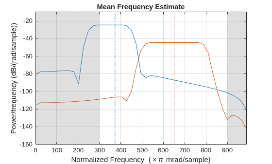
Figure contains an axes object. The axes object with title Mean Frequency Estimate, xlabel Normalized Frequency ( times pi mrad/sample), ylabel Power/frequency (dB/(rad/sample)) contains 6 objects of type line, patch.

Output the mean frequency of each channel. Divide by π.

mnf = meanfreq(d,[],[0.3 0.9]*pi)/pi
mnf = 1×2

    0.3730    0.6500

Since R2026b

Generate a timetable that comprises a three-second quadratic swept-frequency cosine signal with a sample rate of 1 kHz. The frequency sweeping ranges from 150 Hz to 350 Hz.

fs = 1000;
t = (1/fs:1/fs:3)';
f1 = 150;
f2 = 350;
sg = chirp(t,f1,t(end),f2,"quadratic") + 1e-3*randn(size(t));

sgTT = timetable(sg,SampleRate=fs);

Estimate the mean frequency of the signal timetable. Plot the PSD and annotate the mean frequency.

meanfreq(sgTT);
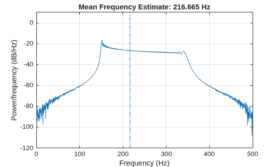
Figure contains an axes object. The axes object with title Mean Frequency Estimate: 216.665 Hz, xlabel Frequency (Hz), ylabel Power/frequency (dB/Hz) contains 2 objects of type line.

You can estimate the mean frequency of the input signal timetable. Remove one sample from the signal timetable every 0.1 seconds.

sgTT(mod(seconds(sgTT.Time),0.1)<1/(2*fs), :) = [];

Estimate the mean frequency of the modified timetable. Plot the PSD and annotate the mean frequency. The estimated mean-frequency value approximates well with the mean-frequency estimation from the unmodified timetable.

meanfreq(sgTT);
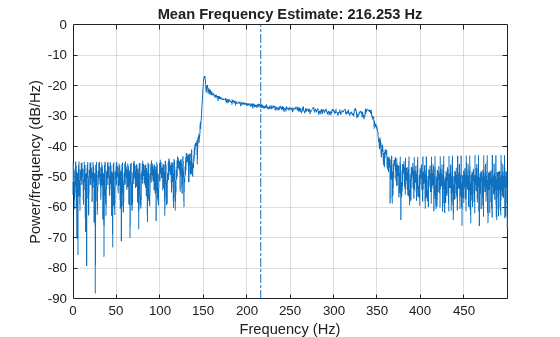
Figure contains an axes object. The axes object with title Mean Frequency Estimate: 216.253 Hz, xlabel Frequency (Hz), ylabel Power/frequency (dB/Hz) contains 2 objects of type line.

Input Arguments

collapse all

Time Domain

Input signal, specified as a real-valued vector, matrix, or timetable.

  • If x is a vector, then the function treats x as a single-channel signal.

  • If x is a matrix or timetable, then meanfreq computes the median frequency of each column or variable independently.

  • You can specify x as a nonuniformly sampled timetable. (since R2026b)

  • x must be finite-valued.

Note

If you specify x as a nonuniformly sampled signal, then meanfreq estimates an effective sample rate and performs uniform resampling before transforming the signal into the frequency domain. You can specify x as a nonuniformly sampled signal if the associated times tv satisfy these conditions:

  • median(diff(tv))/mean(diff(tv)) < 100

  • mean(diff(tv))/median(diff(tv)) < 100

The meanfreq function obtains tv either from x.Time property if x is a timetable or from t if x is a vector or matrix.

Example: cos(pi/4*(0:159))+randn(1,160) is a single-channel row-vector signal.

Example: cos(pi./[4;2]*(0:159))'+randn(160,2) is a two-channel signal.

Data Types: single | double

Sample rate, specified as [] (empty) or a positive scalar.

  • []meanfreq uses normalized frequencies in π rad/sample.

  • Positive scalar — Use a sample rate, which is the number of samples per unit time. If the time is measured in seconds, then the sample rate is in hertz.

This argument does not apply if x is a timetable.

Data Types: single | double

Since R2026b

Sample time, specified as a duration scalar.

This argument does not apply if x is a timetable.

Data Types: duration

Since R2026b

Times associated with the input signal, specified as a vector of nonnegative scalars, a duration vector, or a datetime vector. The function uses the value specified in this argument as the times associated with the vector or matrix x.

  • If x is a vector, then x and t must have the same number of elements.

  • If x is a matrix, then the number of rows in x and the number of elements in t must coincide.

  • You can specify t with nonuniformly spaced elements. In this case, t represents the times associated with a nonuniformly sampled signal x.

This argument does not apply if x is a timetable

Data Types: single | double | duration | datetime

Frequency Domain

Power spectral density (PSD), specified as a vector or matrix. If pxx is a matrix, then meanfreq computes the mean frequency of each column of pxx independently.

The power spectral density must be expressed in linear units, not decibels. Use db2pow to convert decibel values to power values.

Example: [pxx,f] = periodogram(cos(pi./[4;2]*(0:159))'+randn(160,2)) specifies the periodogram PSD estimate of a noisy two-channel sinusoid sampled at 2π Hz and the frequencies at which it is computed.

Data Types: single | double

Frequencies, specified as a vector.

Data Types: single | double

Power spectrum estimate, specified as a vector or matrix. If sxx is a matrix, then meanfreq computes the mean frequency of each column of sxx independently.

The power spectrum must be expressed in linear units, not decibels. Use db2pow to convert decibel values to power values.

Example: [sxx,w] = periodogram(cos(pi./[4;2]*(0:159))'+randn(160,2),'power') specifies the periodogram power spectrum estimate of a two-channel sinusoid embedded in white Gaussian noise and the normalized frequencies at which it is computed.

Data Types: single | double

Resolution bandwidth, specified as a positive scalar. The resolution bandwidth is the product of two values: the frequency resolution of the discrete Fourier transform and the equivalent noise bandwidth of the window used to compute the PSD.

Data Types: single | double

Additional Options

Frequency range, specified as a two-element vector of real values. If you do not specify freqRange, then meanfreq uses the entire bandwidth of the input signal.

Data Types: single | double

Since R2026b

Signal domain, specified as either of these values:

  • "frequency" — The function computes the median frequency from the PSD estimate (pxx) or power spectrum estimate (sxx).

  • "time" — The function computes the mean frequency from the time-domain input signal x.

    Note

    Specify Domain="time" to distinguish time-domain inputs (x,t) from frequency-domain inputs (pxx,f).

Data Types: char | string

Output Arguments

collapse all

Mean frequency, specified as a scalar or vector.

  • If you specify a sample rate, then fMean has the same units as Fs.

  • If you do not specify a sample rate, then fMean has units of rad/sample.

Band power, returned as a scalar or vector.

Algorithms

To determine the mean frequency, meanfreq computes a periodogram power spectrum estimate using a rectangular window. You can obtain the same value of median frequency, fMed, from a signal x at a sample rate Fs in these three ways.

Directly from the signal
fMed = medfreq(x,Fs)
From the periodogram of the signal
[P,F] = periodogram(x,[],length(x),Fs);
fMed = medfreq(P,F)
From the power spectral estimate (Welch's PSD) of the signal
[P,F] = pwelch(x,rectwin(length(x)),[],length(x),Fs);
fMed = medfreq(P,F)

Note

Because meanfreq uses an intermediary representation to transform the input signal from the time domain to frequency domain, the returned median frequency might vary, depending on the signal transformation method, number of DFT points, and window size.

References

[1] Phinyomark, Angkoon, Sirinee Thongpanja, Huosheng Hu, Pornchai Phukpattaranont, and Chusak Limsakul. "The Usefulness of Mean and Median Frequencies in Electromyography Analysis." In Computational Intelligence in Electromyography Analysis – A Perspective on Current Applications and Future Challenges, edited by Ganesh R. Naik. London: IntechOpen, 2012. https://doi.org/10.5772/50639.

Extended Capabilities

expand all

C/C++ Code Generation
Generate C and C++ code using MATLAB® Coder™.

GPU Code Generation
Generate CUDA® code for NVIDIA® GPUs using GPU Coder™.

Version History

Introduced in R2015a

expand all