Linearize DC-DC Converter Model

Model Overview

Open the LinearizeDCDCConverter model.

myModel = "LinearizeDCDCConverter";
open_system(myModel)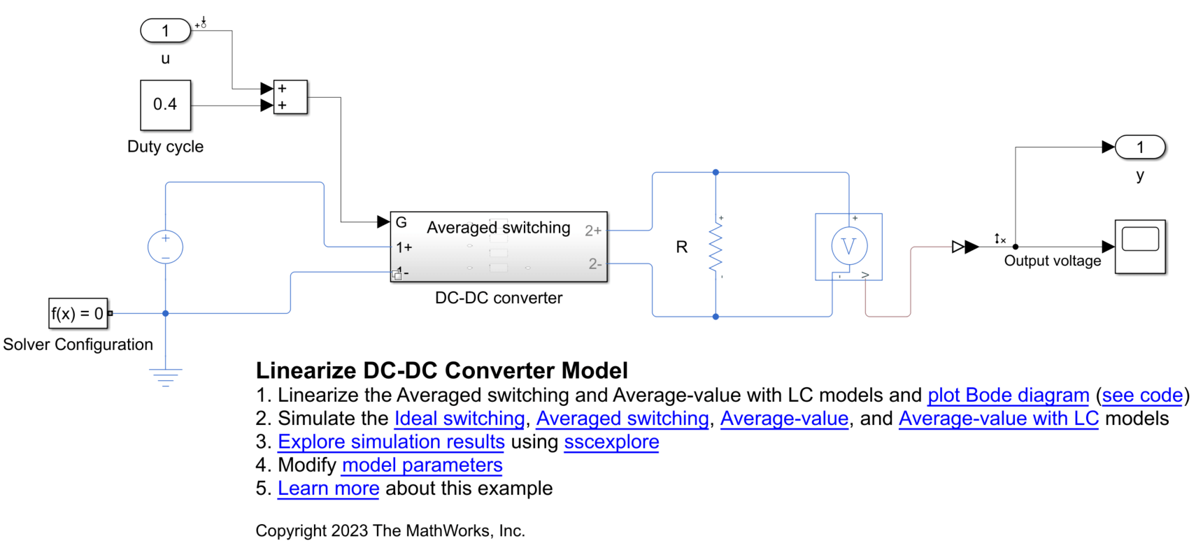

In this example, you model a boost converter using the DC-DC converter subsystem. The DC Voltage Source block supplies 48 V to the converter and the Constant block specifies the duty cycle of the pulse-width modulation (PWM) input to the converter.

Model-Level Inputs and Outputs

To obtain a nontrivial linearized input-output model and generate a frequency response, you must specify model-level inputs and outputs.

In this example, you use the linmod function to linearize the model. To use linmod, you must define top-level or model-level inputs and outputs using Inport and Outport blocks, respectively. The corresponding ports of the top-level model are u and y, respectively.

The linmod function provides basic linearization functionality. For full linearization functionality, use Simulink Control Design™ software. Simulink Control Design™ software requires that you specify input and output signal lines with linearization points. The specified lines must be Simulink signal lines, not Simscape™ physical connection lines. The top-level model specifies these linearization points. If you have Simulink Control Design™ software installed, you can follow the steps in this example to prepare the model for linearization and then use other techniques to linearize the model. For more information about different tools that you can use to linearize models, see Choose Linearization Tools (Simulink Control Design).

Solver Configuration

To linearize the model, you must clear the Use local solver parameter in the Solver Configuration block.

You can select the Start simulation from steady state parameter to start the simulation from a steady state so that the solution at time zero is a suitable operating point for linearization.

DC-DC Converter Model Variant Subsystem

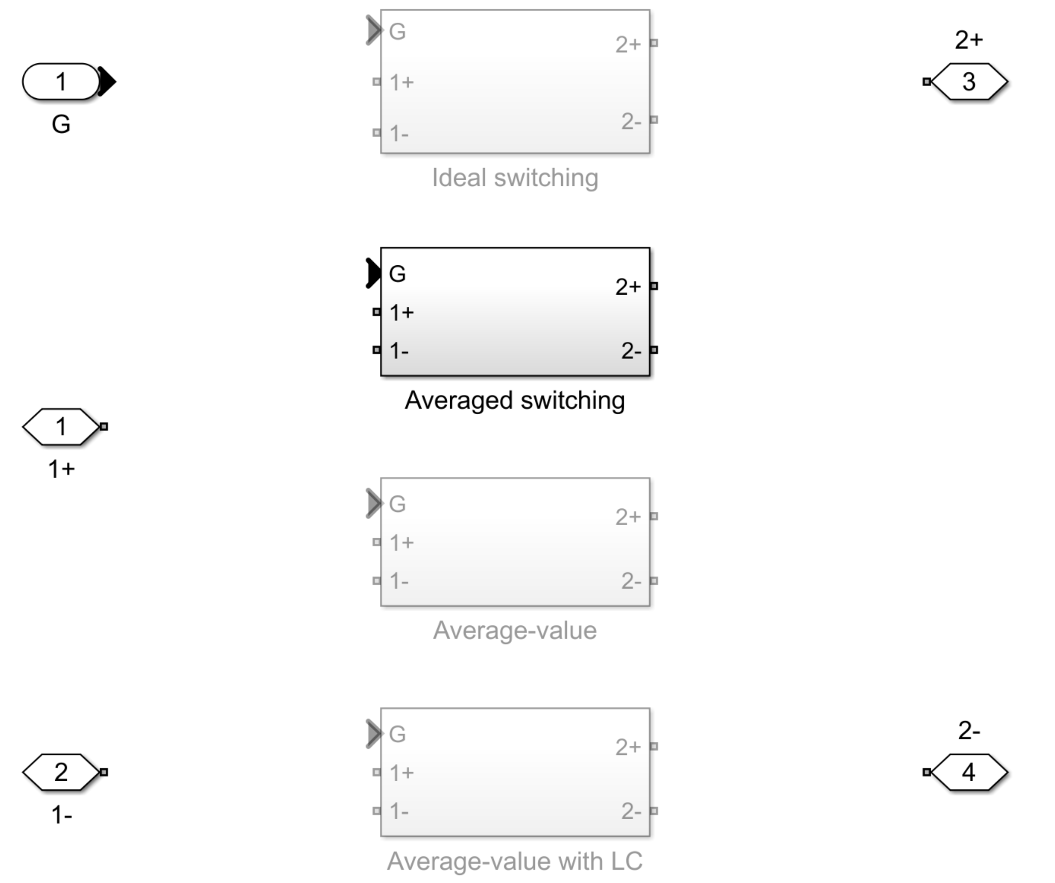
You can use variant subsystems to include multiple implementations of a model in a separate hierarchy. In this example, you implement four models of the boost converter as separate subsystems inside the DC-DC converter subsystem and switch between the subsystems using variant controls. For more information, see Variant Subsystem and Introduction to Variant Controls. To use the Ideal switching, Averaged switching, Average-value, or Average-value with LC subsystem for the simulation, set the activeVariant workspace variable to "Ideal switching", "Averaged switching", "Average-value", or "Average-value with LC", respectively.

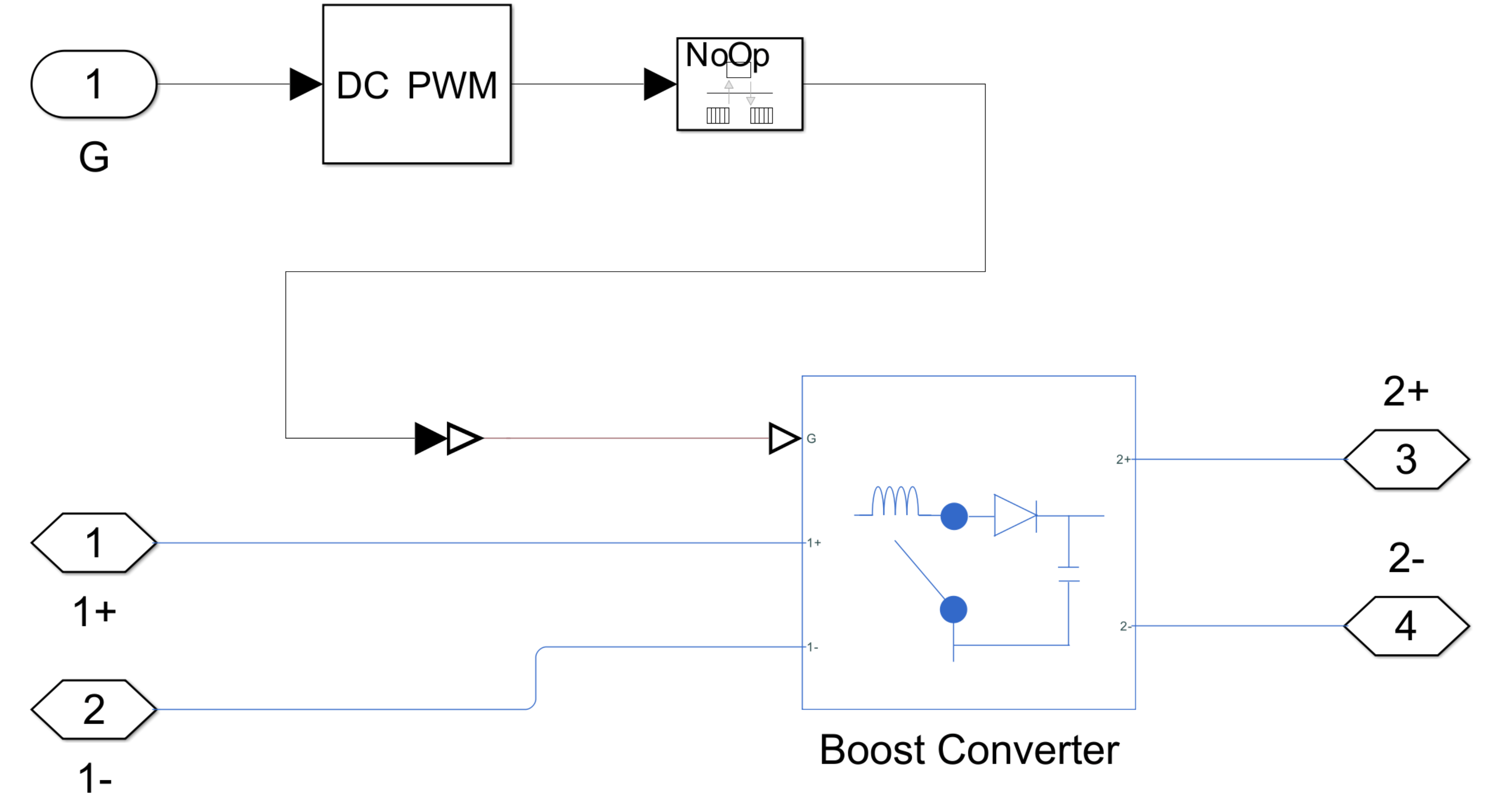
The Ideal switching subsystem is a high-fidelity, piecewise-linear model of the converter. You can use this model for converter-level modeling. To create this model, you can use a Boost Converter block and set the Modeling option parameter to Nonsynchronous converter. Set the Switching device parameter to Ideal semiconductor switch. Then, use PWM Generator and Rate Transition blocks to implement a PWM signal, which you can input to the control signal port G.

You cannot linearize this model exactly because the PWM signal contains strong discontinuities. If you attempt to linearize the model exactly, the model linearizes to zero gain. Furthermore, if you find a linear approximation to your model from simulation results, the approximation is valid only over a small time interval because the output voltage oscillates significantly even when the model reaches a statistically steady state. The solution is to use a lower-fidelity model for the converter without the PWM input signal.

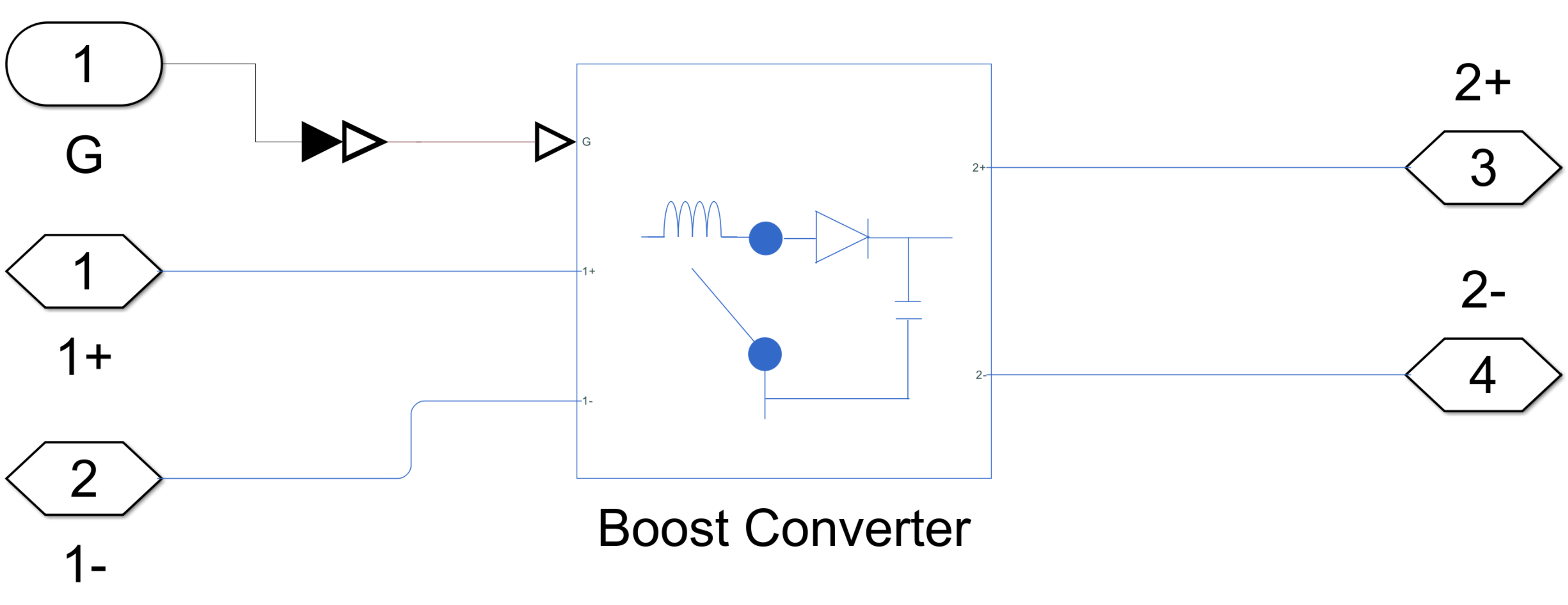
The Averaged switching subsystem is a medium-fidelity model of the converter. You can use this model for subsystem-level modeling. To create this model, you can use a Boost Converter block and set the Switching device parameter to Averaged Switch. When you set the Switching device parameter to Averaged Switch, the control signal port G accepts values in the interval [0, 1]. When G is 0 or 1, the averaged switch is fully opened or fully closed, respectively. The switch behaves similarly to the Ideal Semiconductor Switch block with an antiparallel diode. When G is between 0 and 1, the averaged switch is partly opened. You can then average the PWM signal over a specified period. With an averaged signal, you can use modulation waveforms instead of PWM signals. Input a constant equal to the duty cycle to the control signal port G.

You can linearize this model exactly.

The Average-value subsystem is a low-fidelity model of the converter. You can use this model for system-level modeling. To create this model, you can use an Average-Value DC-DC Converter block and set the Converter type parameter to Boost converter.

You can linearize models with average-value converters exactly. However, if the system does not model any dynamics between the model-level input and output, the results reflect only the limiting behavior of the converter at low frequencies. This situation occurs with the Average-value model because the Average-Value DC-DC Converter block models a converter without an inductor or capacitor. You can introduce dynamics to the model by adding Inductor block and Capacitor blocks.

The Average-value with LC subsystem is a low-fidelity model of the converter that includes an inductor and a capacitor. To create this model, you can use an Average-Value DC-DC Converter block and set the Converter type parameter to Boost converter. Then, connect Inductor and Capacitor blocks to the Average-Value DC-DC Converter block. To obtain comparable results to the Average switching model, set the Inductance and Series resistance parameters of the Capacitor block to the values you specify for the Inductance and Inductor series resistance parameters of the Boost Converter block, respectively. Then, set the Capacitance and Series Resistance parameters of the Capacitor block to the values you specify for the Capacitance and Capacitor effective series resistance parameters of the Boost Converter block, respectively.

You can linearize this model exactly.

Plot Output Voltage of Ideal Switching Model

To get a more comprehensive understanding of the converter behavior and how the output voltage approaches a steady state, run a transient simulation of the high-fidelity model.

To set the active subsystem to Ideal switching for the simulation, set activeVariant to "Ideal switching".

activeVariant = "Ideal switching";

In the Solver Configuration block, clear the Start simulation from steady state parameter.

SimscapeSolver = myModel + "/Solver Configuration";
set_param(SimscapeSolver,DoDC="off");

Simulate the model and plot the evolution of the output voltage over time. The circuit starts from its initial nonsteady state, and the output voltage approaches and eventually settles into a steady oscillation. The output voltage is DC in the sense that the polarity is constant. However, the voltage varies significantly with time. If you find a linear approximation to this model from simulation results, the approximation is valid only over a small time interval because the output voltage oscillates significantly even when the model reaches a statistically steady state.

sim(myModel)
voltage = LinearizeDCDCConverterSimlog.Voltage_Sensor.V.series.values;
time = LinearizeDCDCConverterSimlog.Voltage_Sensor.V.series.time;

figure
plot(time,voltage)
ylim ([0 100])
title("Ideal Switching")
xlabel("Time (s)")
ylabel("Output Voltage (V)")

Prepare Model for Linearization Using Averaged Switching

To find a linear approximation of models with discontinuities, you first need to approximate the discontinuous signal with a continuous approximation.

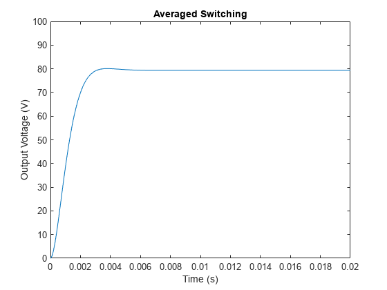
To prepare the model for linearization, set the active subsystem to Averaged switching for the simulation. Activating this subsystem sets the Switching device parameter of the Boost Converter block to Averaged Switch and replaces the discontinuous PWM signal with a constant equal to the duty cycle. Set activeVariant to "Averaged switching".

activeVariant = "Averaged switching";

Simulate the model and plot the evolution of the output voltage over time. The circuit starts from its initial nonsteady state, and the output voltage approaches and eventually reaches a constant value. This steady-state solution is a suitable operating point for linearization.

sim(myModel)
voltage = LinearizeDCDCConverterSimlog.Voltage_Sensor.V.series.values;
time = LinearizeDCDCConverterSimlog.Voltage_Sensor.V.series.time;

figure
plot(time,voltage)
ylim ([0 100])
title("Averaged Switching")
xlabel("Time (s)")
ylabel("Output Voltage (V)")

By default, the linmod function linearizes the model at time zero. You can use the steady-state solver to start the simulation from a steady state. Alternatively, you can define a new operating point.

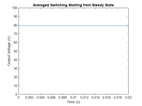
Select the Start simulation from steady state parameter in the Solver Configuration block. When you select this parameter, the solver attempts to find the steady state that results from holding the system inputs constant for a sufficiently long time.

set_param(SimscapeSolver,DoDC="on");

Simulate the model and plot the evolution of the output voltage over time. The output voltage is constant from the start of the simulation. You can linearize the model exactly at time zero.

sim(myModel)
voltage = LinearizeDCDCConverterSimlog.Voltage_Sensor.V.series.values;
time = LinearizeDCDCConverterSimlog.Voltage_Sensor.V.series.time;

figure
plot(time,voltage)
ylim ([0 100])
title("Averaged Switching Starting from Steady State")
xlabel("Time (s)")
ylabel("Output Voltage (V)")

Linearize Averaged Switching Model and Plot Frequency Response

Linearize the model using the linmod function.

[a,b,c,d] = linmod(myModel);

To visualize the results, plot a Bode diagram. If you have a Control System Toolbox™ or Simulink Control Design™ license, you can easily plot a Bode Diagram using the bode (Control System Toolbox) function or Model Linearizer (Simulink Control Design) app, respectively. For more information about different techniques that you can use to create a Bode plot for small-signal frequency-domain analysis, see the Linearize an Electronic Circuit example.

For this example, plot the Bode diagram without using Control System Toolbox™ or Simulink Control Design™ software. Compute the open-loop transfer function G from the state-space representation matrices A, B, C, and D.

npts = 100;
f = logspace(0,8,npts);
G = zeros(1,npts);

for i = 1:npts                                                       
    G(i) = c*(2*pi*1i*f(i)*eye(size(a))-a)^-1*b + d;
end

Calculate the magnitude and phase from the open-loop transfer function and plot the Bode diagram.

figure
subplot(2,1,1), semilogx(f,20*log10(abs(G))) 
grid
title("Bode Diagram")
xlabel("Frequency (Hz)")
ylabel("Magnitude (dB)")

subplot(2,1,2), semilogx(f,180/pi*unwrap(angle(G)))
grid
xlabel("Frequency (Hz)")
ylabel("Phase (degree)")                                          

Prepare Model for Linearization Using Average-Value Converter

As an alternative to using blocks that support the Averaged switch option, you can use low-fidelity, average-value converter blocks. To model a boost converter, you can use an Average-Value DC-DC Converter block and set the Converter type parameter to boost converter.

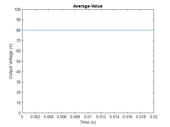
To set the active subsystem to Average-value for the simulation, set activeVariant to "Average-value".

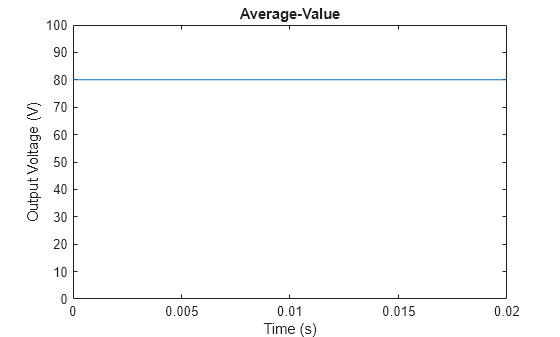
activeVariant = "Average-value";

Simulate the model and plot the evolution of the output voltage over time. The output voltage is close to the output voltage of the Averaged switching model.

sim(myModel)
voltage = LinearizeDCDCConverterSimlog.Voltage_Sensor.V.series.values;
time = LinearizeDCDCConverterSimlog.Voltage_Sensor.V.series.time;

figure()
plot(time,voltage)
ylim ([0 100])
title("Average-Value")
xlabel("Time (s)")
ylabel("Output Voltage (V)")

Linearize the model.

[a,b,c,d] = linmod(myModel);

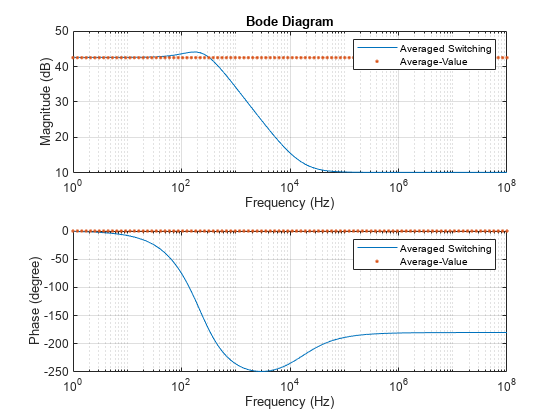
Calculate the magnitude and phase from the state-space representations and plot the Bode diagram. The model agrees with the Averaged switching model at low frequencies but is unable to accurately capture the high-frequency dynamics of the system because the system does not model any dynamics between the model-level input and output.

GAverageValue = zeros(1,npts);

for i = 1:npts                                                       
    GAverageValue(i) = c*(2*pi*1i*f(i)*eye(size(a))-a)^-1*b + d;
end

figure()
subplot(2,1,1), semilogx(f,20*log10(abs(G))) 
hold on
semilogx(f,20*log10(abs(GAverageValue)),".")
hold off
grid
title("Bode Diagram")
xlabel("Frequency (Hz)")
ylabel("Magnitude (dB)")
legend("Averaged Switching","Average-Value")

subplot(2,1,2), semilogx(f,180/pi*unwrap(angle(G)))
hold on
semilogx(f,180/pi*unwrap(angle(GAverageValue)),".")
grid
xlabel("Frequency (Hz)")
ylabel("Phase (degree)")                                          
legend("Averaged Switching","Average-Value")

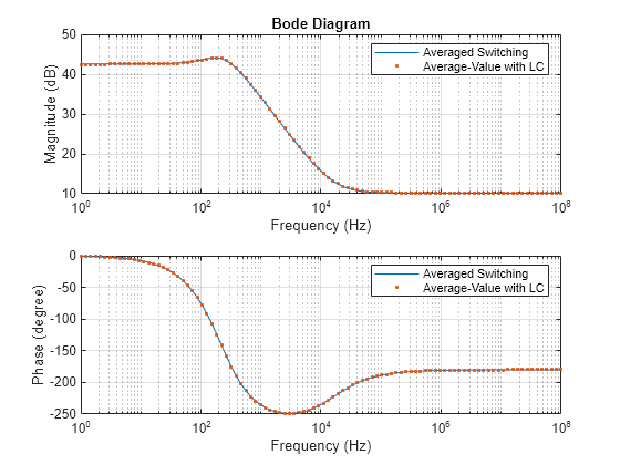
Include Inductor and Capacitor blocks in your average-value converter model. To set the active subsystem to Average-value with LC for the simulation, set activeVariant to "Average-value with LC". This system models dynamics between the model-level input and output. You can linearize the model exactly at time zero.

activeVariant = "Average-value with LC";

Linearize Average-Value with LC Model and Plot Frequency Response

Linearize the model.

[a,b,c,d] = linmod(myModel);

Calculate the magnitude and phase from the state-space representations and plot the Bode diagram. The model agrees with the Averaged switching model over the entire frequency range.

GAverageValue = zeros(1,npts);

for i = 1:npts                                                       
    GAverageValue(i) = c*(2*pi*1i*f(i)*eye(size(a))-a)^-1*b + d;
end

figure
subplot(2,1,1), semilogx(f,20*log10(abs(G))) 
hold on
semilogx(f,20*log10(abs(GAverageValue)),".")
hold off
grid
title("Bode Diagram")
xlabel("Frequency (Hz)")
ylabel("Magnitude (dB)")
legend("Averaged Switching","Average-Value with LC")

subplot(2,1,2), semilogx(f,180/pi*unwrap(angle(G)))
hold on
semilogx(f, 180/pi*unwrap(angle(GAverageValue)),".")
hold off
xlabel("Frequency (Hz)")
ylabel("Phase (degree)")                                          
grid
legend("Averaged Switching","Average-Value with LC")