Main Content

dbscan

Density-based spatial clustering of applications with noise (DBSCAN)

Description

idx = dbscan(X,epsilon,minpts) partitions observations in the n-by-p data matrix X into clusters using the DBSCAN algorithm (see Algorithms). dbscan clusters the observations (or points) based on a threshold for a neighborhood search radius epsilon and a minimum number of neighbors minpts required to identify a core point. The function returns an n-by-1 vector (idx) containing cluster indices of each observation.

example

idx = dbscan(X,epsilon,minpts,Name,Value) specifies additional options using one or more name-value pair arguments. For example, you can specify 'Distance','minkowski','P',3 to use the Minkowski distance metric with an exponent of three in the DBSCAN algorithm.

example

idx = dbscan(D,epsilon,minpts,'Distance','precomputed') returns a vector of cluster indices for the precomputed pairwise distances D between observations. D can be the output of pdist or pdist2, or a more general dissimilarity vector or matrix conforming to the output format of pdist or pdist2, respectively.

example

[idx,corepts] = dbscan(___) also returns a logical vector corepts that contains the core points identified by dbscan, using any of the input argument combinations in the previous syntaxes.

example

Examples

collapse all

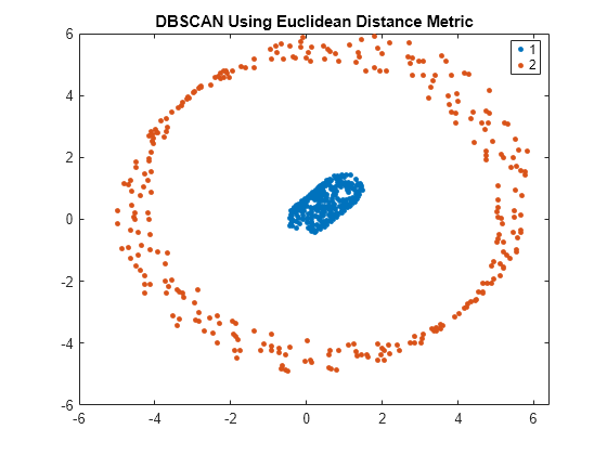
Cluster a 2-D circular data set using DBSCAN with the default Euclidean distance metric. Also, compare the results of clustering the data set using DBSCAN and k-Means clustering with the squared Euclidean distance metric.

Generate synthetic data that contains two noisy circles.

rng('default') % For reproducibility

% Parameters for data generation
N = 300;  % Size of each cluster
r1 = 0.5; % Radius of first circle
r2 = 5;   % Radius of second circle
theta = linspace(0,2*pi,N)';

X1 = r1*[cos(theta),sin(theta)]+ rand(N,1); 
X2 = r2*[cos(theta),sin(theta)]+ rand(N,1);
X = [X1;X2]; % Noisy 2-D circular data set

Visualize the data set.

scatter(X(:,1),X(:,2))

Figure contains an axes object. The axes object contains an object of type scatter.

The plot shows that the data set contains two distinct clusters.

Perform DBSCAN clustering on the data. Specify an epsilon value of 1 and a minpts value of 5.

idx = dbscan(X,1,5); % The default distance metric is Euclidean distance

Visualize the clustering.

gscatter(X(:,1),X(:,2),idx);
title('DBSCAN Using Euclidean Distance Metric')

Figure contains an axes object. The axes object with title DBSCAN Using Euclidean Distance Metric contains 2 objects of type line. One or more of the lines displays its values using only markers These objects represent 1, 2.

Using the Euclidean distance metric, DBSCAN correctly identifies the two clusters in the data set.

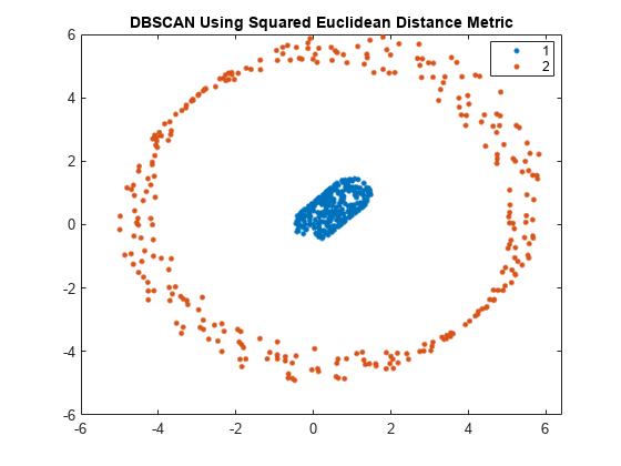
Perform DBSCAN clustering using the squared Euclidean distance metric. Specify an epsilon value of 1 and a minpts value of 5.

idx2 = dbscan(X,1,5,'Distance','squaredeuclidean');

Visualize the clustering.

gscatter(X(:,1),X(:,2),idx2);
title('DBSCAN Using Squared Euclidean Distance Metric')

Figure contains an axes object. The axes object with title DBSCAN Using Squared Euclidean Distance Metric contains 2 objects of type line. One or more of the lines displays its values using only markers These objects represent 1, 2.

Using the squared Euclidean distance metric, DBSCAN correctly identifies the two clusters in the data set.

Perform k-Means clustering using the squared Euclidean distance metric. Specify k = 2 clusters.

kidx = kmeans(X,2); % The default distance metric is squared Euclidean distance

Visualize the clustering.

gscatter(X(:,1),X(:,2),kidx);
title('K-Means Using Squared Euclidean Distance Metric')

Figure contains an axes object. The axes object with title K-Means Using Squared Euclidean Distance Metric contains 2 objects of type line. One or more of the lines displays its values using only markers These objects represent 1, 2.

Using the squared Euclidean distance metric, k-Means clustering fails to correctly identify the two clusters in the data set.

Perform DBSCAN clustering using a matrix of pairwise distances between observations as input to the dbscan function, and find the number of outliers and core points. The data set is a Lidar scan, stored as a collection of 3-D points, that contains the coordinates of objects surrounding a vehicle.

Load the x, y, z coordinates of the objects.

load('lidar_subset.mat') 
loc = lidar_subset;

To highlight the environment around the vehicle, set the region of interest to span 20 meters to the left and right of the vehicle, 20 meters in front and back of the vehicle, and the area above the surface of the road.

xBound = 20; % in meters
yBound = 20; % in meters
zLowerBound = 0; % in meters

Crop the data to contain only points within the specified region.

indices = loc(:,1) <= xBound & loc(:,1) >= -xBound ...
    & loc(:,2) <= yBound & loc(:,2) >= -yBound ...
    & loc(:,3) > zLowerBound;
loc = loc(indices,:);

Visualize the data as a 2-D scatter plot. Annotate the plot to highlight the vehicle.

scatter(loc(:,1),loc(:,2),'.');
annotation('ellipse',[0.48 0.48 .1 .1],'Color','red')

Figure contains an axes object. The axes object contains an object of type scatter.

The center of the set of points (circled in red) contains the roof and hood of the vehicle. All other points are obstacles.

Precompute a matrix of pairwise distances D between observations by using the pdist2 function.

D = pdist2(loc,loc);

Cluster the data by using dbscan with the pairwise distances. Specify an epsilon value of 2 and a minpts value of 50.

[idx, corepts] = dbscan(D,2,50,'Distance','precomputed');

Visualize the results and annotate the figure to highlight a specific cluster.

numGroups = length(unique(idx));
gscatter(loc(:,1),loc(:,2),idx,hsv(numGroups));
annotation('ellipse',[0.54 0.41 .07 .07],'Color','red')
grid

Figure contains an axes object. The axes object contains 12 objects of type line. One or more of the lines displays its values using only markers These objects represent -1, 1, 2, 3, 4, 5, 6, 7, 8, 9, 10, 11.

As shown in the scatter plot, dbscan identifies 11 clusters and places the vehicle in a separate cluster.

dbscan assigns the group of points circled in red (and centered around (3,–4)) to the same cluster (group 7) as the group of points in the southeast quadrant of the plot. The expectation is that these groups should be in separate clusters. You can try using a smaller value of epsilon to split up large clusters and further partition the points.

The function also identifies some outliers (an idx value of –1 ) in the data. Find the number of points that dbscan identifies as outliers.

sum(idx == -1)
ans = 
412

dbscan identifies 412 outliers out of 19,070 observations.

Find the number of points that dbscan identifies as core points. A corepts value of 1 indicates a core point.

sum(corepts == 1)
ans = 
18446

dbscan identifies 18,446 observations as core points.

See Determine Values for DBSCAN Parameters for a more extensive example.

Input Arguments

collapse all

Input data, specified as an n-by-p numeric matrix. The rows of X correspond to observations (or points), and the columns correspond to variables.

Data Types: single | double

Pairwise distances between observations, specified as a numeric row vector that is the output of pdist, numeric square matrix that is the output of pdist2, logical row vector, or logical square matrix. D can also be a more general dissimilarity vector or matrix that conforms to the output format of pdist or pdist2, respectively.

For the aforementioned specifications, the following table describes the formats that D can take, given an input matrix X that has n observations (rows) and p dimensions (columns).

SpecificationFormat
Numeric row vector (output of pdist(X))
  • A row vector of length n(n – 1)/2, corresponding to pairs of observations in X

  • Distances arranged in the order (2,1), (3,1), ..., (n,1), (3,2), ..., (n,2), ..., (n,n – 1))

Numeric square matrix (output of pdist2(X,X))
  • An n-by-n matrix, where D(i,j) is the distance between observations i and j in X

  • A symmetric matrix having diagonal elements equal to zero

Logical row vector
  • A row vector of length n(n – 1)/2, corresponding to pairs of observations in X

  • A logical row vector with elements indicating distances that are less than or equal to epsilon

  • Elements of D arranged in the order (2,1), (3,1), ..., (n,1), (3,2), ..., (n,2), ..., (n,n – 1))

Logical square matrix
  • An n-by-n matrix, where D(i,j) indicates the distance between observations i and j in X that are less than or equal to epsilon

Note

If D is a logical vector or matrix, then the value of epsilon must be empty; for example, dbscan(D,[],5,'Distance','precomputed').

Data Types: single | double | logical

Epsilon neighborhood of a point, specified as a numeric scalar that defines a neighborhood search radius around the point. If the epsilon neighborhood of a point contains at least minpts neighbors, then dbscan identifies the point as a core point.

The value of epsilon must be empty ([]) when D is a logical vector or matrix.

Example: dbscan(X,2.5,10)

Example: dbscan(D,[],5,'Distance','precomputed'), for a logical matrix or vector D

Data Types: single | double

Minimum number of neighbors required for a core point, specified as a positive integer. The epsilon neighborhood of a core point in a cluster must contain at least minpts neighbors, whereas the epsilon neighborhood of a border point can contain fewer neighbors than minpts.

Example: dbscan(X,2.5,5)

Data Types: single | double

Name-Value Arguments

Specify optional pairs of arguments as Name1=Value1,...,NameN=ValueN, where Name is the argument name and Value is the corresponding value. Name-value arguments must appear after other arguments, but the order of the pairs does not matter.

Before R2021a, use commas to separate each name and value, and enclose Name in quotes.

Example: dbscan(D,2.5,5,'Distance','precomputed') specifies DBSCAN clustering using a precomputed matrix of pairwise distances D between observations, an epsilon neighborhood of 2.5, and a minimum of 5 neighbors.

Distance metric, specified as the comma-separated pair consisting of 'Distance' and a character vector, string scalar, or function handle, as described in this table.

ValueDescription
'precomputed'

Precomputed distances. You must specify this option if the first input to dbscan is a vector or matrix of pairwise distances D.

'euclidean'

Euclidean distance (default)

'squaredeuclidean'

Squared Euclidean distance. (This option is provided for efficiency only. It does not satisfy the triangle inequality.)

'seuclidean'

Standardized Euclidean distance. Each coordinate difference between observations is scaled by dividing by the corresponding element of the standard deviation, S = std(X,'omitnan'). Use Scale to specify another value for S.

'mahalanobis'

Mahalanobis distance using the sample covariance of X, C = cov(X,'omitrows'). Use Cov to specify another value for C, where the matrix C is symmetric and positive definite.

'cityblock'

City block distance

'minkowski'

Minkowski distance. The default exponent is 2. Use P to specify a different exponent, where P is a positive scalar value.

'chebychev'

Chebychev distance (maximum coordinate difference)

'cosine'

One minus the cosine of the included angle between points (treated as vectors)

'correlation'

One minus the sample correlation between points (treated as sequences of values)

'hamming'

Hamming distance, which is the percentage of coordinates that differ

'jaccard'

One minus the Jaccard coefficient, which is the percentage of nonzero coordinates that differ

'spearman'

One minus the sample Spearman's rank correlation between observations (treated as sequences of values)

@distfun

Custom distance function handle. A distance function has the form

function D2 = distfun(ZI,ZJ)
% calculation of distance
...
where

  • ZI is a 1-by-n vector containing a single observation.

  • ZJ is an m2-by-n matrix containing multiple observations. distfun must accept a matrix ZJ with an arbitrary number of observations.

  • D2 is an m2-by-1 vector of distances, and D2(k) is the distance between observations ZI and ZJ(k,:).

If your data is not sparse, you can generally compute distance more quickly by using a built-in distance instead of a function handle.

For definitions, see Distance Metrics.

When you use the 'seuclidean', 'minkowski', or 'mahalanobis' distance metric, you can specify the additional name-value pair argument 'Scale', 'P', or 'Cov', respectively, to control the distance metrics.

Example: dbscan(X,2.5,5,'Distance','minkowski','P',3) specifies an epsilon neighborhood of 2.5, a minimum of 5 neighbors to grow a cluster, and use of the Minkowski distance metric with an exponent of 3 when performing the clustering algorithm.

Exponent for the Minkowski distance metric, specified as the comma-separated pair consisting of 'P' and a positive scalar.

This argument is valid only if 'Distance' is 'minkowski'.

Example: 'P',3

Data Types: single | double

Covariance matrix for the Mahalanobis distance metric, specified as the comma-separated pair consisting of 'Cov' and a symmetric, positive definite, numeric matrix.

This argument is valid only if 'Distance' is 'mahalanobis'.

Data Types: single | double

Scaling factors for the standardized Euclidean distance metric, specified as the comma-separated pair consisting of 'Scale' and a numeric vector of positive values.

Each dimension (column) of X has a corresponding value in 'Scale'; therefore, 'Scale' is of length p (the number of columns in X). For each dimension of X, dbscan uses the corresponding value in 'Scale' to standardize the difference between X and a query point.

This argument is valid only if 'Distance' is 'seuclidean'.

Data Types: single | double

Output Arguments

collapse all

Cluster indices, returned as a numeric column vector. idx has n rows, and each row of idx indicates the cluster assignment of the corresponding observation in X. An index equal to –1 indicates an outlier (or noise point).

Note

Cluster assignment using the DBSCAN algorithm is dependent on the order of observations. Therefore, shuffling the rows of X can lead to different cluster assignments for the observations. For more details, see Algorithms.

Data Types: double

Indicator for core points, returned as an n-by-1 logical vector indicating the indices of the core points identified by dbscan. A value of 1 in any row of corepts indicates that the corresponding observation in X is a core point. Otherwise, corepts has a value of 0 for rows corresponding to observations that are not core points.

Data Types: logical

More About

collapse all

Core Points

Core points in a cluster are points that have at least a minimum number of neighbors (minpts) in their epsilon neighborhood (epsilon). Each cluster must contain at least one core point.

Border Points

Border points in a cluster are points that have fewer than the required minimum number of neighbors for a core point (minpts) in their epsilon neighborhood (epsilon). Generally, the epsilon neighborhood of a border point contains significantly fewer points than the epsilon neighborhood of a core point.

Noise Points

Noise points are outliers that do not belong to any cluster.

Tips

  • For improved speed when iterating over many values of epsilon, consider passing in D as the input to dbscan. This approach prevents the function from having to compute the distances at every point of the iteration.

  • If you use pdist2 to precompute D, do not specify the 'Smallest' or 'Largest' name-value pair arguments of pdist2 to select or sort columns of D. Selecting fewer than n distances results in an error, because dbscan expects D to be a square matrix. Sorting the distances in each column of D leads to a loss in the interpretation of D and can give meaningless results when used in the dbscan function.

  • For efficient memory usage, consider passing in D as a logical matrix rather than a numeric matrix to dbscan when D is large. By default, MATLAB® stores each value in a numeric matrix using 8 bytes (64 bits), and each value in a logical matrix using 1 byte (8 bits).

  • To select a value for minpts, consider a value greater than or equal to the number of dimensions of the input data plus one [1]. For example, for an n-by-p matrix X, set 'minpts' equal to p+1 or greater.

  • One possible strategy for selecting a value for epsilon is to generate a k-distance graph for X. For each point in X, find the distance to the kth nearest point, and plot sorted points against this distance. Generally, the graph contains a knee. The distance that corresponds to the knee is typically a good choice for epsilon, because it is the region where points start tailing off into outlier (noise) territory [1].

Algorithms

  • DBSCAN is a density-based clustering algorithm that is designed to discover clusters and noise in data. The algorithm identifies three kinds of points: core points, border points, and noise points [1]. For specified values of epsilon and minpts, the dbscan function implements the algorithm as follows:

    1. From the input data set X, select the first unlabeled observation x1 as the current point, and initialize the first cluster label C to 1.

    2. Find the set of points within the epsilon neighborhood epsilon of the current point. These points are the neighbors.

      1. If the number of neighbors is less than minpts, then label the current point as a noise point (or an outlier). Go to step 4.

        Note

        dbscan can reassign noise points to clusters if the noise points later satisfy the constraints set by epsilon and minpts from some other point in X. This process of reassigning points happens for border points of a cluster.

      2. Otherwise, label the current point as a core point belonging to cluster C.

    3. Iterate over each neighbor (new current point) and repeat step 2 until no new neighbors are found that can be labeled as belonging to the current cluster C.

    4. Select the next unlabeled point in X as the current point, and increase the cluster count by 1.

    5. Repeat steps 2–4 until all points in X are labeled.

  • If two clusters have varying densities and are close to each other, that is, the distance between two border points (one from each cluster) is less than epsilon, then dbscan can merge the two clusters into one.

  • Every valid cluster might not contain at least minpts observations. For example, dbscan can identify a border point belonging to two clusters that are close to each other. In such a situation, the algorithm assigns the border point to the first discovered cluster. As a result, the second cluster is still a valid cluster, but it can have fewer than minpts observations.

References

[1] Ester, M., H.-P. Kriegel, J. Sander, and X. Xiaowei. “A density-based algorithm for discovering clusters in large spatial databases with noise.” In Proceedings of the Second International Conference on Knowledge Discovery in Databases and Data Mining, 226-231. Portland, OR: AAAI Press, 1996.

Extended Capabilities

Version History

Introduced in R2019a