Main Content

plsregress

Partial least-squares (PLS) regression

Description

[XL,YL] = plsregress(X,Y,ncomp) returns the predictor and response loadings XL and YL, respectively, for a partial least-squares (PLS) regression of the responses in matrix Y on the predictors in matrix X, using ncomp PLS components.

[XL,YL,XS,YS,BETA,PCTVAR,MSE,stats] = plsregress(X,Y,ncomp) also returns:

  • The predictor scores XS. Predictor scores are PLS components that are linear combinations of the variables in X.

  • The response scores YS. Response scores are linear combinations of the responses with which the PLS components XS have maximum covariance.

  • The matrix BETA of coefficient estimates for the PLS regression model.

  • The percentage of variance PCTVAR explained by the regression model.

  • The estimated mean squared errors MSE for PLS models with ncomp components.

  • A structure stats that contains the PLS weights, T2 statistic, and predictor and response residuals.

example

[XL,YL,XS,YS,BETA,PCTVAR,MSE,stats] = plsregress(___,Name,Value) specifies options using one or more name-value arguments in addition to any of the input argument combinations in previous syntaxes. The name-value arguments specify MSE calculation parameters. For example, 'CV',5 calculates the MSE using 5-fold cross-validation.

Examples

collapse all

Load the spectra data set. Create the predictor X as a numeric matrix that contains the near infrared (NIR) spectral intensities of 60 samples of gasoline at 401 wavelengths. Create the response y as a numeric vector that contains the corresponding octane ratings.

load spectra
X = NIR;
y = octane;

Perform PLS regression with 10 components of the responses in y on the predictors in X.

[XL,yl,XS,YS,beta,PCTVAR] = plsregress(X,y,10);

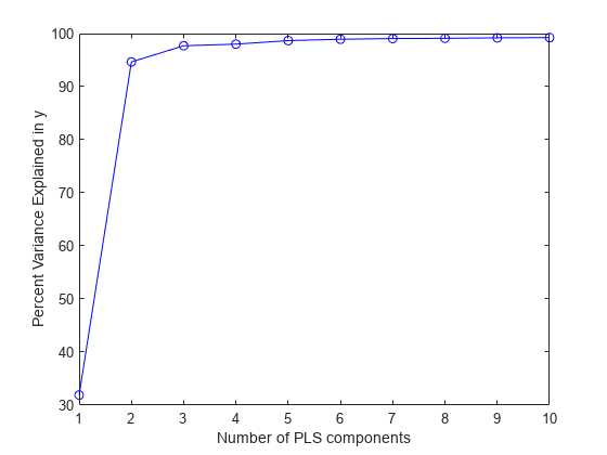
Plot the percent of variance explained in the response variable (PCTVAR) as a function of the number of components.

plot(1:10,cumsum(100*PCTVAR(2,:)),'-bo');
xlabel('Number of PLS components');
ylabel('Percent Variance Explained in y');

Figure contains an axes object. The axes object with xlabel Number of PLS components, ylabel Percent Variance Explained in y contains an object of type line.

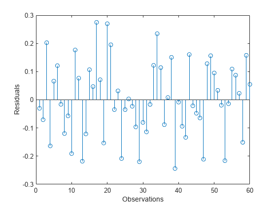
Compute the fitted response and display the residuals.

yfit = [ones(size(X,1),1) X]*beta;
residuals = y - yfit;
stem(residuals)
xlabel('Observations');
ylabel('Residuals');

Figure contains an axes object. The axes object with xlabel Observations, ylabel Residuals contains an object of type stem.

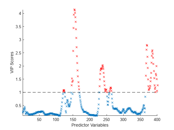
Calculate variable importance in projection (VIP) scores for a partial least-squares (PLS) regression model. You can use VIP to select predictor variables when multicollinearity exists among variables. Variables with a VIP score greater than 1 are considered important for the projection of the PLS regression model [3].

Load the spectra data set. Create the predictor X as a numeric matrix that contains the near infrared (NIR) spectral intensities of 60 samples of gasoline at 401 wavelengths. Create the response y as a numeric vector that contains the corresponding octane ratings. Specify the number of components ncomp.

load spectra
X = NIR;
y = octane;
ncomp = 10;

Perform PLS regression with 10 components of the responses in y on the predictors in X.

[XL,yl,XS,YS,beta,PCTVAR,MSE,stats] = plsregress(X,y,ncomp);

Calculate the normalized PLS weights.

W0 = stats.W ./ sqrt(sum(stats.W.^2,1));

Calculate the VIP scores for ncomp components.

p = size(XL,1);
sumSq = sum(XS.^2,1).*sum(yl.^2,1);
vipScore = sqrt(p* sum(sumSq.*(W0.^2),2) ./ sum(sumSq,2));

Find variables with a VIP score greater than or equal to 1.

indVIP = find(vipScore >= 1);

Plot the VIP scores.

scatter(1:length(vipScore),vipScore,'x')
hold on
scatter(indVIP,vipScore(indVIP),'rx')
plot([1 length(vipScore)],[1 1],'--k')
hold off
axis tight
xlabel('Predictor Variables')
ylabel('VIP Scores')

Figure contains an axes object. The axes object with xlabel Predictor Variables, ylabel VIP Scores contains 3 objects of type scatter, line.

Input Arguments

collapse all

Predictor variables, specified as a numeric matrix. X is an n-by-p matrix, where n is the number of observations and p is the number of predictor variables. Each row of X represents one observation, and each column represents one variable. X must have the same number of rows as Y.

Data Types: single | double

Response variables, specified as a numeric matrix. Y is an n-by-m matrix, where n is the number of observations and m is the number of response variables. Each row of Y represents one observation, and each column represents one variable. Each row in Y is the response for the corresponding row in X.

Data Types: single | double

Number of components, specified as a numeric vector. If you do not specify ncomp, the default value is min(size(X,1) – 1,size(X,2)).

Data Types: single | double

Name-Value Arguments

Specify optional pairs of arguments as Name1=Value1,...,NameN=ValueN, where Name is the argument name and Value is the corresponding value. Name-value arguments must appear after other arguments, but the order of the pairs does not matter.

Before R2021a, use commas to separate each name and value, and enclose Name in quotes.

Example: 'CV',10,'Options',statset('UseParallel',true) calculates the MSE using 10-fold cross-validation, where computations run in parallel.

MSE calculation method, specified as 'resubstitution', a positive integer, or a cvpartition object.

  • Specify 'CV' as 'resubstitution' to use both X and Y to fit the model and estimate the mean squared errors, without cross-validation.

  • Specify 'CV' as a positive integer k to use k-fold cross-validation.

  • Specify 'CV' as a cvpartition object to specify another type of cross-validation partition.

Example: 'CV',5

Example: 'CV',cvpartition(n,'Holdout',0.3)

Data Types: single | double | char | string

Indicator for including the constant term (intercept) in the model fit, specified as true to include the constant term or false to omit it.

Example: 'Intercept',false

Data Types: logical

Number of Monte Carlo repetitions for cross-validation, specified as a positive integer.

  • If you specify CV as 'resubstitution', then the MCReps value must be 1.

  • If you specify CV as a custom cvpartition object (that is, the IsCustom property is set to 1), then the MCReps value must be 1.

Example: 'MCReps',5

Data Types: single | double

Options for computing in parallel and setting random streams, specified as a structure. Create the Options structure using statset. This table lists the option fields and their values.

Field NameValueDefault
UseParallelSet this value to true to run computations in parallel.false
UseSubstreams

Set this value to true to run computations in a reproducible manner.

To compute reproducibly, set Streams to a type that allows substreams: "mlfg6331_64" or "mrg32k3a".

false
StreamsSpecify this value as a RandStream object or cell array of such objects. Use a single object except when the UseParallel value is true and the UseSubstreams value is false. In that case, use a cell array that has the same size as the parallel pool.If you do not specify Streams, then plsregress uses the default stream or streams.

Note

You need Parallel Computing Toolbox™ to run computations in parallel.

Example: Options=statset(UseParallel=true,UseSubstreams=true,Streams=RandStream("mlfg6331_64"))

Data Types: struct

Output Arguments

collapse all

Predictor loadings, returned as a numeric matrix. XL is a p-by-ncomp matrix, where p is the number of predictor variables and ncomp is the number of PLS components. Each row of XL contains coefficients that define a linear combination of PLS components approximating the original predictor variables.

Data Types: single | double

Response loadings, returned as a numeric matrix. YL is an m-by-ncomp matrix, where m is the number of response variables and ncomp is the number of PLS components. Each row of YL contains coefficients that define a linear combination of PLS components approximating the original response variables.

Data Types: single | double

Predictor scores, returned as a numeric matrix. XS is an n-by-ncomp orthonormal matrix, where n is the number of observations and ncomp is the number of PLS components. Each row of XS corresponds to one observation, and each column corresponds to one component.

Data Types: single | double

Response scores, returned as a numeric matrix. YS is an n-by-ncomp matrix, where n is the number of observations and ncomp is the number of PLS components. Each row of YS corresponds to one observation, and each column corresponds to one component. YS is not orthogonal or normalized.

Data Types: single | double

Coefficient estimates for the PLS regression model, returned as a numeric matrix. If the model includes the constant term (intercept), BETA is a (p + 1)-by-m matrix, where p is the number of predictor variables, m is the number of response variables, and the first row of BETA contains the constant term. If the constant term (intercept) is not included, BETA is a p-by-m matrix.

Data Types: single | double

Percentage of variance explained by the model, returned as a numeric matrix. PCTVAR is a 2-by-ncomp matrix, where ncomp is the number of PLS components. The first row of PCTVAR contains the percentage of variance explained in X by each PLS component, and the second row contains the percentage of variance explained in Y.

Data Types: single | double

Mean squared error, returned as a numeric matrix. MSE is a 2-by-(ncomp + 1) matrix, where ncomp is the number of PLS components. MSE contains the estimated mean squared errors for a PLS model with ncomp components. The first row of MSE contains mean squared errors for the predictor variables in X, and the second row contains mean squared errors for the response variables in Y. The column j of MSE contains mean squared errors for j – 1 components.

Data Types: single | double

Model statistics, returned as a structure with the fields described in this table.

FieldDescription
Wp-by-ncomp matrix of PLS weights so that XS = X0*W
T2T2 statistic for each point in XS
XresidualsPredictor residuals, X0 – XS*XL'
YresidualsResponse residuals, Y0 – XS*YL'

For more information about the centered predictor and response variables X0 and Y0, see Algorithms.

Algorithms

plsregress uses the SIMPLS algorithm [1]. If the model fit includes the constant term (intercept), the function first centers X and Y by subtracting the column means to get the centered predictor and response variables X0 and Y0, respectively. However, the function does not rescale the columns. To perform PLS regression with standardized variables, use zscore to normalize X and Y (columns of X0 and Y0 are centered to have mean 0 and scaled to have standard deviation 1).

After centering X and Y, plsregress computes the singular value decomposition (SVD) on X0'*Y0. The predictor and response loadings XL and YL are the coefficients obtained from regressing X0 and Y0 on the predictor score XS. You can reconstruct the centered data X0 and Y0 using XS*XL' and XS*YL', respectively.

plsregress initially computes YS as YS = Y0*YL. By convention [1], however, plsregress then orthogonalizes each column of YS with respect to preceding columns of XS, so that XS'*YS is a lower triangular matrix.

If the model fit does not include the constant term (intercept), X and Y are not centered as part of the fitting process.

References

[1] de Jong, Sijmen. “SIMPLS: An Alternative Approach to Partial Least Squares Regression.” Chemometrics and Intelligent Laboratory Systems 18, no. 3 (March 1993): 251–63. https://doi.org/10.1016/0169-7439(93)85002-X.

[2] Rosipal, Roman, and Nicole Kramer. "Overview and Recent Advances in Partial Least Squares." Subspace, Latent Structure and Feature Selection: Statistical and Optimization Perspectives Workshop (SLSFS 2005), Revised Selected Papers (Lecture Notes in Computer Science 3940). Berlin, Germany: Springer-Verlag, 2006, vol. 3940, pp. 34–51. https://doi.org/10.1007/11752790_2.

[3] Chong, Il-Gyo, and Chi-Hyuck Jun. “Performance of Some Variable Selection Methods When Multicollinearity Is Present.” Chemometrics and Intelligent Laboratory Systems 78, no. 1–2 (July 2005) 103–12. https://doi.org/10.1016/j.chemolab.2004.12.011.

Extended Capabilities

Version History

Introduced in R2008a