Survey Urban Environment Using UAV
This example shows how to specify a coverage region for a UAV and capture its flight data while surveying an urban environment. To map its environment, the UAV flies through a city and captures aerial images using a camera and other sensor data.
Specify Coverage Space for UAV
Create a coverage space for the UAV by providing it with these points in order:
A takeoff position.
Vertices of the coverage area polygon in order.
A landing position.
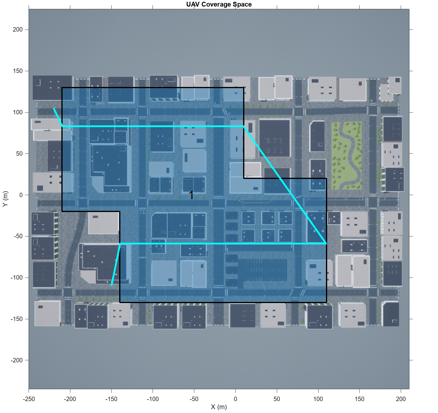
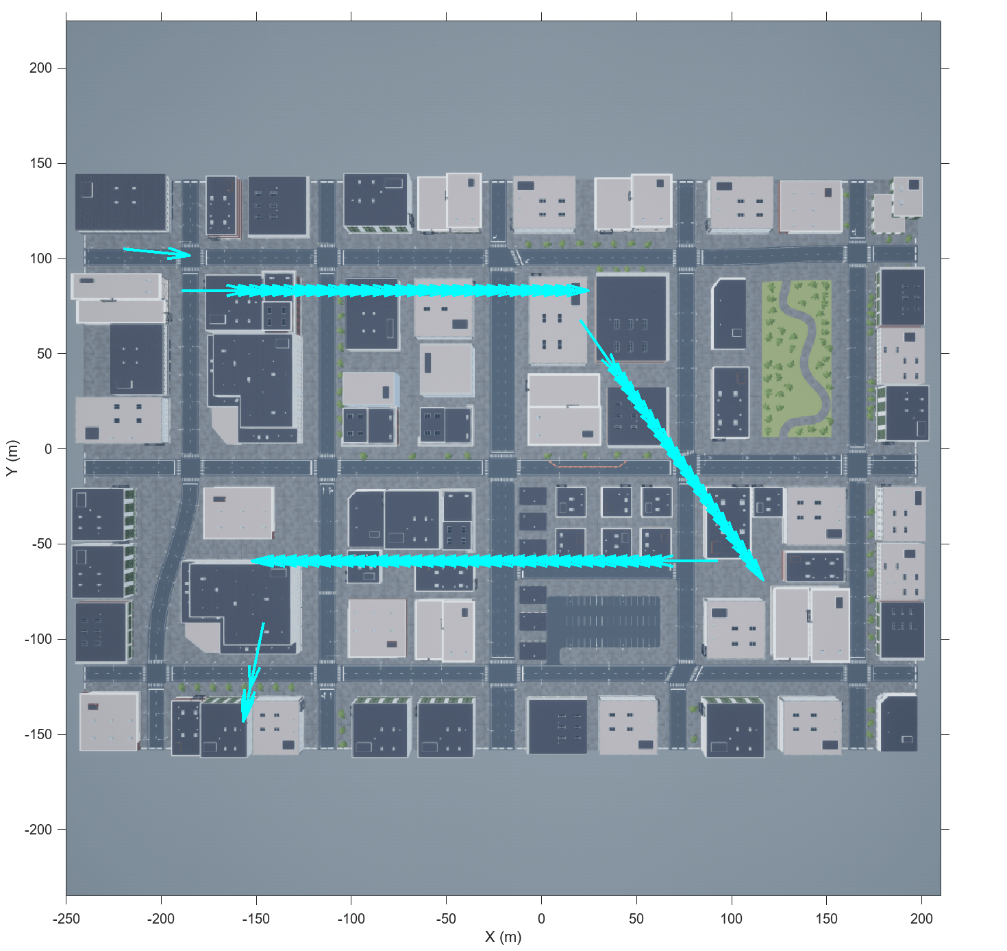
Since the map used in this example is from the Unreal Engine® US City Block scene, the positions of each point must be with respect to the world frame of that scene. This image shows a top view of the scene with the desired coverage space, along with the takeoff and landing positions.

The flight path must:
Takeoff at point T at an xyz-position of
[-220 -105 0].Fly through a planned path covering the polygonal region enclosed within points 1-8.
Land at point L at an *xyz-*position of
[-150 -110 0].
The takeoff and landing points have elevations of 0 meters, but you must specify heights for waypoints 1-8.
Specify a target elevation for the UAV. The UAV must maintain this elevation for the entire flight.
targetUAVElevation = 150;
Specify the focal length, in pixels, along the X and Y axes of the camera. You will use a symmetrical lens with the same focal length along both axes.
focalLengthX = 1109;
focalLengthY = focalLengthX;
Specify the width and height, in pixels, of the image captured by the camera. It is assumed that the optical center is at the geometric center of this image plane.
imageWidth = 1024;
imageHeight = 512;
Calculate the coverage width for the uavCoveragePlanner using the camera parameters and UAV elevation. First, compute the vertical and horizontal fields of view of the camera.
fovHorizontal = 2*atan(imageWidth/(2*focalLengthY));
fovVertical = 2*atan(imageHeight/(2*focalLengthX));
Then compute the coverage width. Refer to the Appendix section for more information on these formulae.
coverageWidth = (2*targetUAVElevation*tan(fovHorizontal/2))/sin(pi/2 + fovVertical/2);
Set takeoff position, xy only.
takeoff = [-220, 105];
Set vertices of the polygonal region to be covered, in order, xy only.
regionVertices = [-210,130;
                10,130;
                10,20;
               110,20;
               110,-130;
              -140,-130;
              -140,-20;
              -210,-20];
Set landing position, xy only.
landing = [-150, -110];
Compute Trajectory Using Coverage Planner
First, show the US City Block scene with axes limits in meters.
Load the spatial reference limits of the scene.
load('USCityBlockSpatialReference.mat');Show US City Block scene. Flip the image before plotting the axes since the y-axis is also being flipped.
figure
fileName = 'USCityBlock.jpg';
cityBlock = flip(imread(fileName),1);
imshow(cityBlock,spatialReference)
set(gca,'YDir','normal')
xlabel('X (m)')
ylabel('Y (m)')
The coverage width that you have calculated and coverage height together make up the coverage area of the UAV. The coverage area is the area of the ground plane captured by the UAV's camera per image. These values can be used to compute a coverage plan for the UAV to ensure the entire area of interest, called the coverage space, is fully covered.
Create a coverage space using the vertices and drone elevation defined above.
cs = uavCoverageSpace(Polygons=regionVertices,UnitWidth=coverageWidth,ReferenceHeight=targetUAVElevation);
Display the coverage space.
hold on
show(cs);
title("UAV Coverage Space")
hold off
Now, compute the coverage waypoints using the takeoff, coverage space and landing positions.
Takeoff = [takeoff 0];
Landing = [landing 0];
cp = uavCoveragePlanner(cs);
[waypoints,~] = cp.plan(Takeoff,Landing);
Show the computed path as an animated line.
hold on
h = animatedline;
h.Color = "cyan";
h.LineWidth = 3;
for i = 1:size(waypoints,1)
    addpoints(h,waypoints(i,1),waypoints(i,2));
    pause(1);
end
hold off
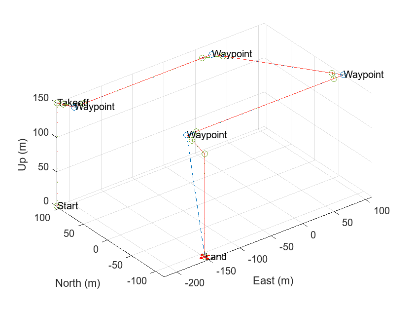
Finally, compute and visualize the flight trajectory of the UAV using the exampleHelperComputeAndShowUAVTrajectory helper function.
[positionTbl,rotationTbl,traj] = exampleHelperComputeAndShowUAVTrajectory(waypoints(:,1:2),targetUAVElevation);
Run Simulation and Obtain Filtered Flight Data
This section uses the Unreal simulation to capture data, and stores the acquired Simulink® signal data in the out MAT file, which contains these outputs:
SimulationMetadata— Metadata from the Simulink simulation.logsout— Logged data acquired by the UAV during its flight. This includes image, label, and depth information.
The simulation finds the time steps at which the UAV is within specific tolerance values for the target elevation and pitch. It then logs data for only those time steps where the yaw velocity is also below its specific tolerance value. This process maintains a central perspective projection at the correct elevation and removes noisy data.
A target pitch of radians has been specified in the Simulink model. This value is in the UAV's local coordinate system. Do not modify this as the next few examples assume this pitch value for their calculations to be accurate.
First, set the tolerance values for camera elevation, drone pitch and camera roll velocity.
elevationTolerance = 15e-2;
pitchTolerance = 2;
rollVelocityTolerance = 1e-4;
Notice that since the camera is pointing downwards, towards the ground, its local reference frame has been rotated by 90 degrees. Hence, we specify the local yaw velocity tolerance for the drone, which in turn is the local roll velocity tolerance for the camera.
Then, filter out every frame. To create a map, you do not need every frame that meets the tolerance requirements. Increasing results in faster, but less accurate, map creation, while decreasing it results in slower, but more accurate, map creation. You must ensure that the successively captured image frames have overlap regions between them. Use an value of 20 so that the captured data meets these requirements.
nthFrame = 20;
Open the mSurveyUrbanEnvironment Simulink model.
pathToModel = "mSurveyUrbanEnvironment";
open_system(pathToModel);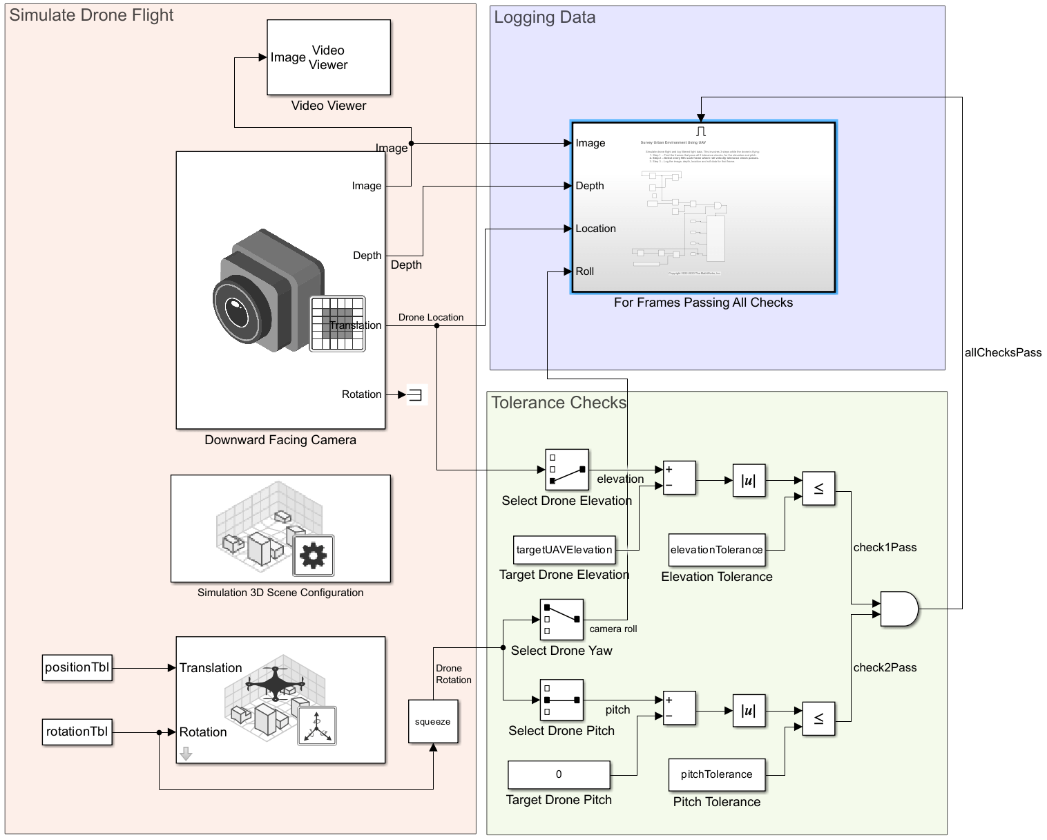
Run the model to start the Unreal Engine simulation and capture the camera images, depth images, drone locations and camera roll data in the out MAT file. Note that you need at least 700 MB of disk space to save the captured simulation data.
sim("mSurveyUrbanEnvironment")
Load Captured Data
Load the out MAT file generated by the Simulink model.
load outThe out MAT file contains this data captured from the model:
Image— Image frames acquired by the UAV camera for each time step, returned as an H-by-W-by-3-by-F array.Depth— Depth map for each image frame acquired by the UAV camera, returned as an H-by-W-by-F array.Roll— Camera roll for each image frame acquired by the UAV camera, returned as an *1-*by-1-by-F array.Location— Location for each image frame acquired by the UAV camera, returned as an 1-by-3-by-F array.
H and W are the height and width, respectively, of the acquired images, in pixels. F is the total number of time steps logged, and is directly proportional to the flight time.
Save the image, depth and location data into workspace variables.
image = logsout.get("Image").Values.Data;
depth = logsout.get("Depth").Values.Data;
liveUAVLocation = logsout.get("Location").Values.Data;
Since camera roll is obtained from a different source block in the model, we need to synchronize it separately from the other acquired data.
Obtain the roll time steps and match it will the image time steps.
[~,matchedSteps] = ismember(logsout.get("Image").Values.Time,logsout.get("Roll").Values.Time);
Now obtain roll only at these matching time steps and save it into a workspace variable.
liveUAVRoll = logsout.get("Roll").Values.Data(matchedSteps);Show Captured Drone Location and Orientation
Show the captured drone location and orientation as a quiver.
First, show the US City Block scene with axes limits in meters.
figure;
imshow(cityBlock,spatialReference);
set(gca,'YDir','normal')
xlabel('X (m)')
ylabel('Y (m)')
Get the X and Y coordinates of the drone when the data was captured. This is the location of the drone.
X = squeeze(liveUAVLocation(1,1,:));
Y = squeeze(liveUAVLocation(1,2,:));
Get the directional components of the drone when the data was captured. This is the orientation of the drone.
U = cos(squeeze(liveUAVRoll));
V = sin(squeeze(liveUAVRoll));
Plot it over the UAV coverage space.
hold on;
quiver(X,Y,U,V,"cyan","LineWidth",2);
hold off;
Save Filtered Data
You must calculate the values of these additional parameters for orthophoto computation:
focalLength— The focal length of the UAV camera, in meters. Note that the UAV camera in this example is facing vertically downward.meterToPixel— The number of pixels on your screen that constitute 1 meter in the real world. This is also the ratio between your screen and the Simulink space.reductionFactor— This value represents the reduction factor for each axis. If the saved orthophoto [H W] size pixels, then the actual size of the orthophoto is [H W]reductionFactorin pixels, and the real-world size of the orthophoto, in meters, is [H W]reductionFactormeterToPixel. This ensures that 1 meter in this final map is equivalent to 1 meter in real life. Because processing matrices with millions of rows and columns is computationally expensive, you use the reduction factor to scale down such matrices.
Obtain the focal length of the camera. Assume a symmetrical lens with the same focal length along the x- and y-axes.
focalLength = focalLengthX;
Calculate the meter-to-pixel ratio for your screen. This initial value is for a screen on which 752 pixels corresponds to 15.6 cm in the real world. If this value does not match those of your screen, determine the ratio for your monitor and set meterToPixel accordingly.
meterToPixel = 752*100/15.6;
Next, set the reduction factor for the orthophoto to 800. Where a reduction factor of 1 results in a 1:1 scale map of the ground, which would be too large to efficiently process, a reduction factor of 800 results in a 1:800 scale map. Note that, depending on your use case, you may need to tune the reduction factor, as high or too low of a value can cause ripple effects in the orthophoto.
reductionFactor = 800;
Save the image, depth, liveUAVRoll and liveUAVLocation data, along with the additional orthophoto parameters, into a MAT file.
save("flightData.mat", ...
    "image","depth","liveUAVRoll","liveUAVLocation", ...
    "targetUAVElevation","meterToPixel","focalLength","reductionFactor", ...
    "-v7.3");
Conclusion
This example showed how to create a flight trajectory for a UAV using coverage planning, simulate the UAV flight, and capture information from the sensors during the UAV flight. It also showed how to only log the data of interest by eliminating noise.
In the next step of the Map and Classify Urban Environment Using UAV Camera and Deep Learning workflow, Obtain Orthophotos from Central Perspective Images, you process the captured perspective images to convert them into orthophotos.
Appendix
In 2 dimensions, the relationship between the field of view, the focal length, and the image height of the camera is illustrated as follows.
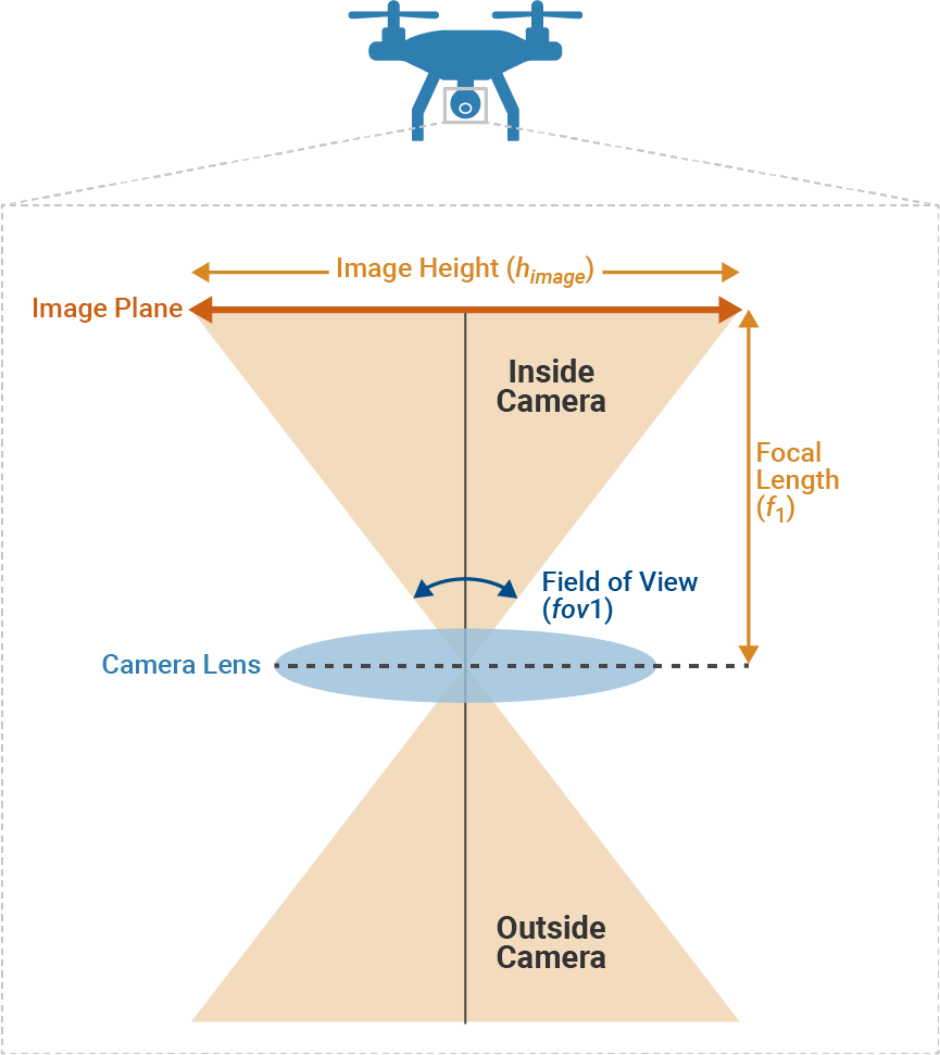
In this view, the camera faces down with a pitch of 0 degrees which allows it to acquire a central perspective image. The area above the camera lens with the image plane lies inside the UAV camera, and the area below the camera lens captures the scene outside the UAV camera.
The field of view along the x-axis of the image plane can be calculated as follows.
Where
is the x-axis focal length of the camera
is the height of the image captured on the image plane inside the camera.
The field of view along the y-axis of the image plane can be calculated using a similar formula.
Where
is the y-axis focal length of the camera
is the width of the image captured on the image plane inside the camera. For a symmetrical lens, = .
In 3 dimensions, the relationship between the field of view, the height of the UAV and the coverage area of the camera [1] is illustrated as follows.
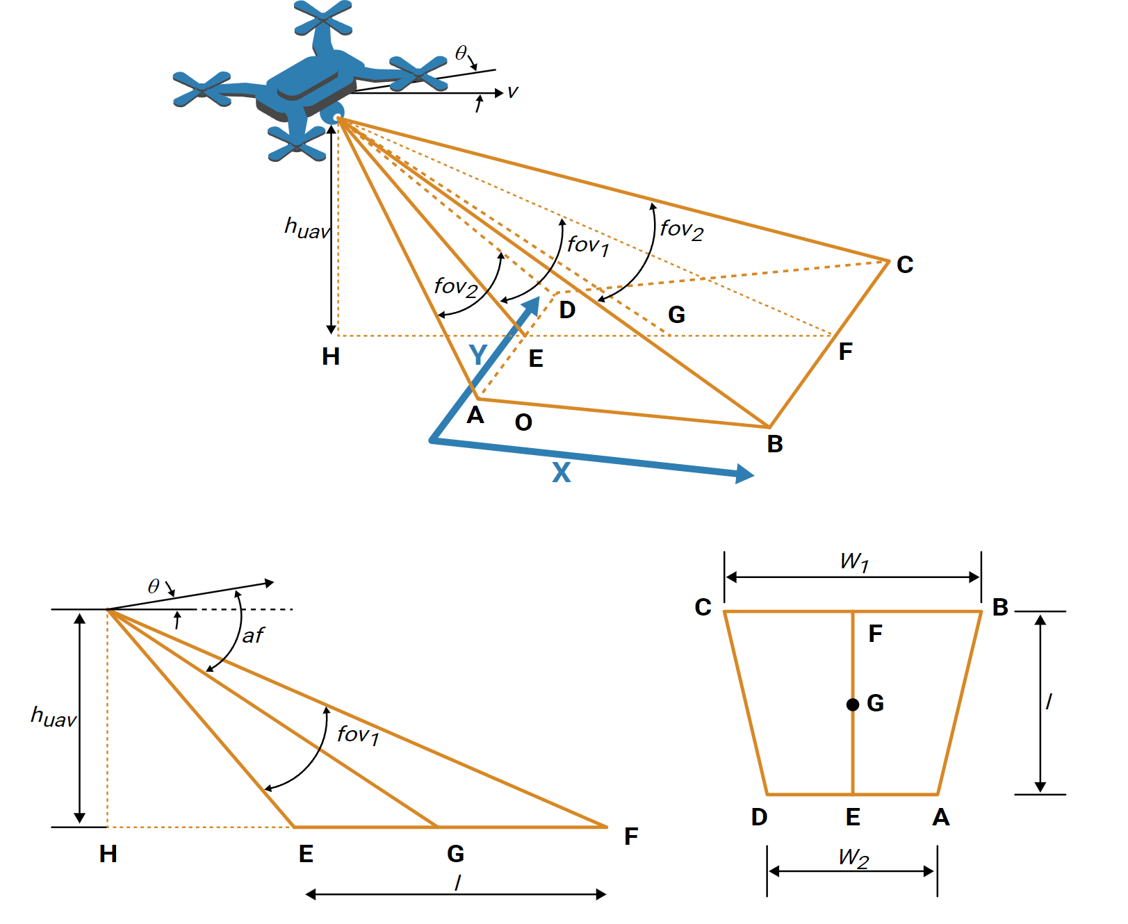
Where is the elevation of the UAV, is the mounting angle of the camera relative to the UAV and is the pitch of the UAV. lies outside the UAV camera and is the coverage area of the UAV.
Based on the above diagram, the coverage width of the camera can be calculated as follows.
In this example, the UAV's camera is facing down with a mounting angle of radians. The UAV also flies parallel to the ground with a pitch of 0 degrees. These assumptions results in the following simplification of the coverage width calculation.
Notice that this also makes which is similar to the values in this example.
References
[1] Li, Yan, Hai Chen, Meng Joo Er, and Xinmin Wang. "Coverage path planning for UAVs based on enhanced exact cellular decomposition method." Mechatronics 21, no. 5 (August 2011): 876-885. https://doi.org/10.1016/j.mechatronics.2010.10.009