Create Orthomosaic from Orthophotos

Background

Feature detection and matching are powerful techniques used in many computer vision applications, such as image registration, tracking, and object detection. In this example, you use feature-based and location-based techniques to automatically stitch together a set of orthophotos. Orthophotos are geometrically corrected images that have a uniform scale, which enables them to be stitched easily with minimal changes.

Image registration is the process of aligning two images into a single integrated image. For more information about the image registration, see Image Registration. The procedure for image stitching is an extension of the feature-based image registration process. Instead of registering a single pair of images, you register multiple image pairs, so that the mapped features align with each other to form an orthomosaic.

Feature-Based Stitching

The process of feature-based stitching of two images is:

1.Take two images and find the matching features between the two images.

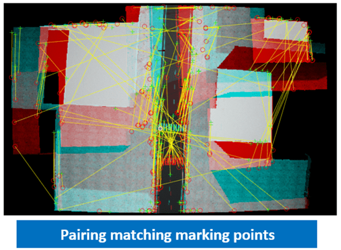
2. Compute the affine transform for image 2, such that its matching features overlap those in image 1.

3. Combine both of the images into a single image with their features overlapping. The resulting image is slightly larger, as it now contains the unique data from both images.

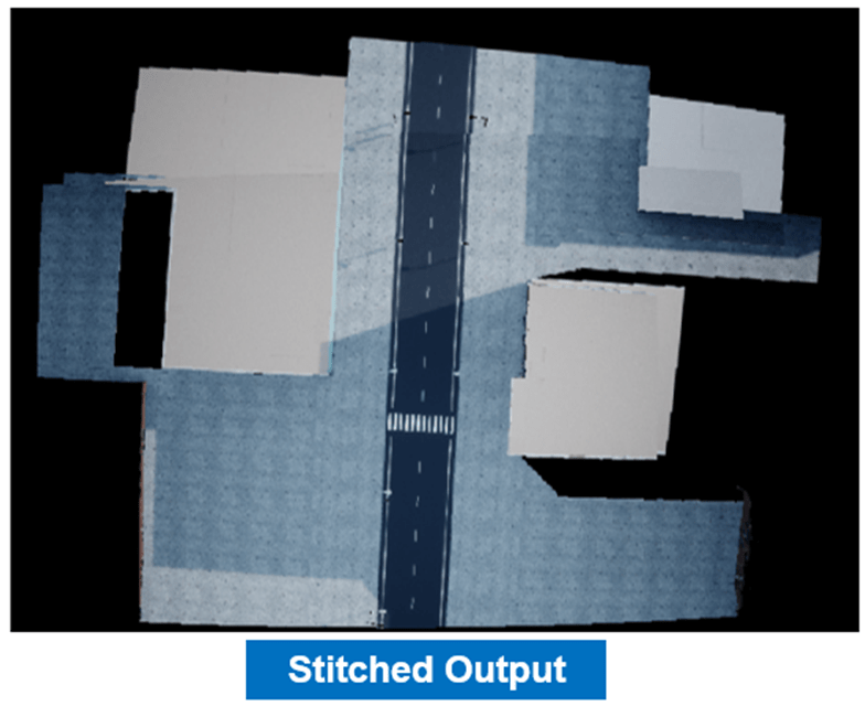
Each time you repeat this process, the stitched output becomes larger, until the final output incorporates the features from all of the images.

Location-Based Stitching

The process of location-based stitching of two images is:

1. Take two images and obtain their corresponding orientation and position as logged by a sensor. In this case the logged roll angle and the position of the drone when the images were captured. Since the yaw, pitch and elevation of drone when the two images were captured were constant, they do not need to be captured for each frame.

2. Rotate the two images by their corresponding roll angles so that their orientations match. Note that the yaw, pitch and elevation of drone when the two images were captured were constant. This ensures that, post rotation by their corresponding roll angle, their scale matches by default.

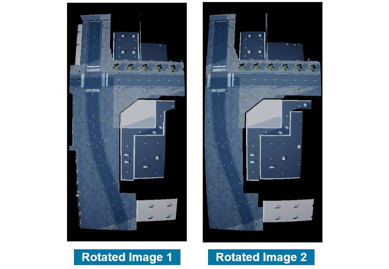
3. The local pitch and yaw of the drone camera being 0 degrees and the camera having a symmetrical lens ensures that the location of the drone is actually the location of the center point of the images when they were captured. We use this information to overlap and hence register the 2 images.

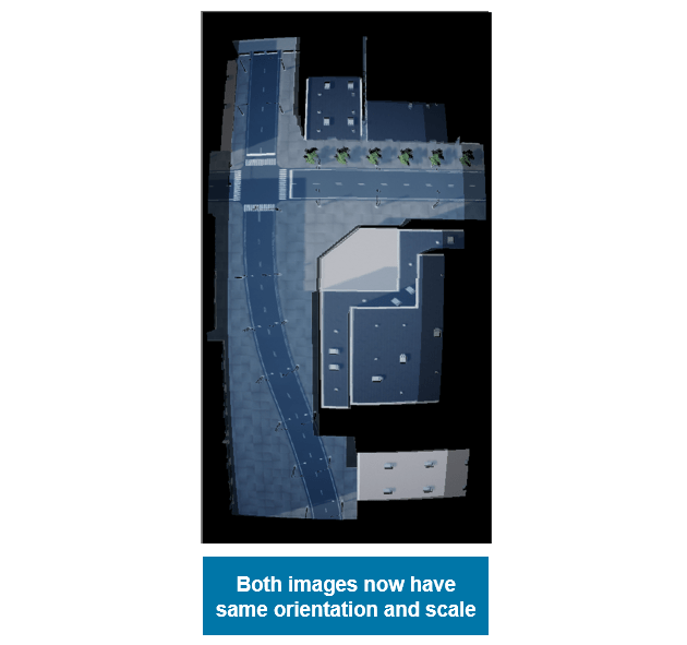
4. Combine both of the images into a single image using their corresponding center locations. The resulting image is slightly larger, as it now contains the unique data from both images.

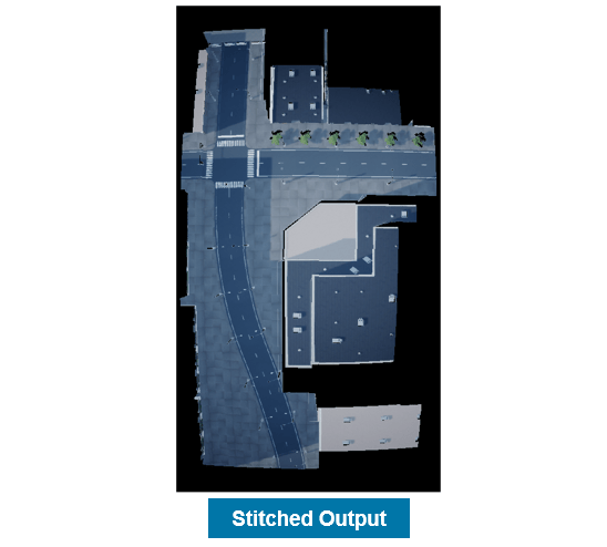
Each time you repeat this process, the stitched output becomes larger, until the final output incorporates the locations from all of the images.

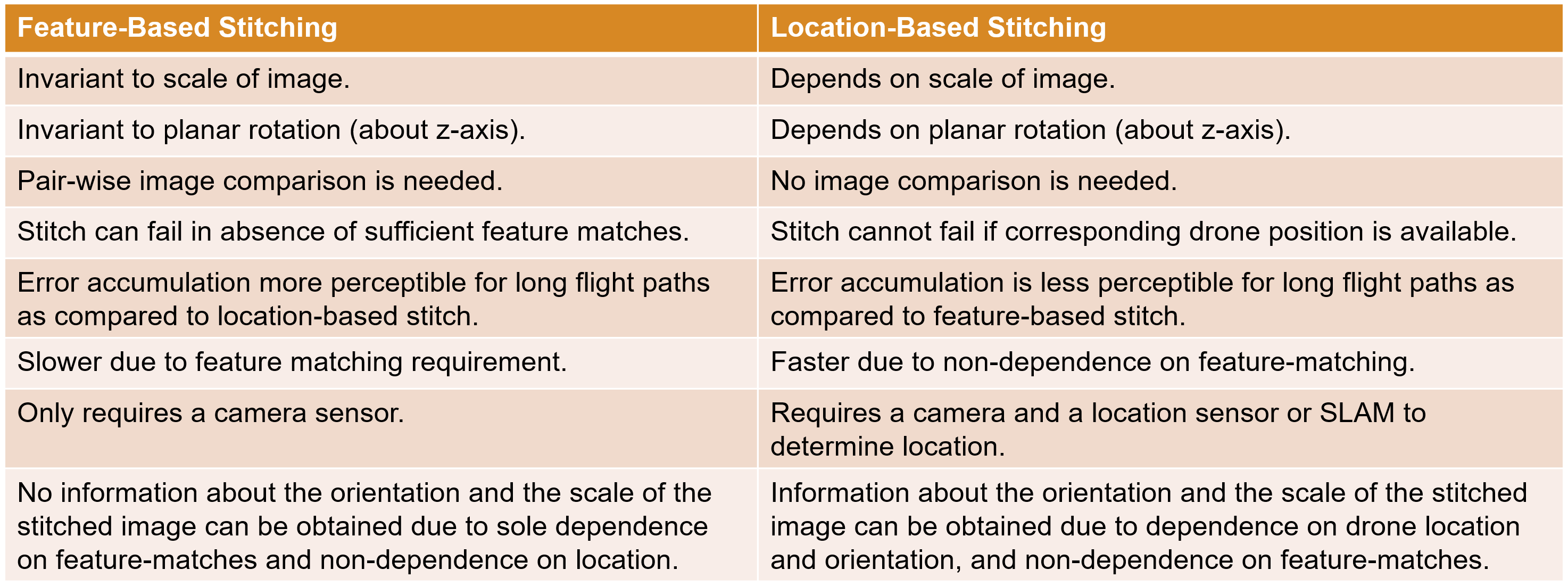
Comparing Stitching Techniques

Setup

If you have not run the Survey Urban Environment Using UAV example, you can download that data for this example by setting ranSurveyEx to false. Otherwise, set ranSurveyEx to true.

ranSurveyEx = "false";

If ranSurveyEx is false, download the required data.

if strcmp(ranSurveyEx,"false")
    preAcquiredDataComponent = "uav/data/R2023b";
    preAcquiredDataFilename = "flightData.zip";
    disp("Downloading previously acquired flight data (300 MB)...");
    preAcquiredDataFolder = exampleHelperDownloadData(preAcquiredDataComponent,preAcquiredDataFilename);
end

Downloading previously acquired flight data (300 MB)...

This example also uses a pretrained Deeplab v3+ network with a Resnet-18 backbone. For more information on the pretrained network, see the previous example Semantic Segmentation of Orthophotos.

The network has been trained for binary semantic segmentation to identify roofs, classified as Roof, and nonroofs, classified as NonRoof.

If you have not run the Semantic Segmentation of Orthophotos example, you can download that data for this example by setting ranSemanticEx to false. Otherwise, set ranSemanticEx to true.

ranSemanticEx = "false";

If ranSemanticEx is false, download the required data.

if strcmp(ranSemanticEx,"false")
    orthoDataComponent = "uav/data/R2023b";
    orthoDataFilename = "orthoData.zip";
    disp("Downloading previously processed orthophotos and ortholabels data (50 MB)...");
    orthoDataFolder = exampleHelperDownloadData(orthoDataComponent,orthoDataFilename);
end

Downloading previously processed orthophotos and ortholabels data (50 MB)...

Download the pretrained network.

pretrainedNetworkComponent = "uav/data";
pretrainedNetworkFilename = "deeplabv3plusResnet18Unreal.zip";
disp("Downloading pretrained network (60 MB) ...");

Downloading pretrained network (60 MB) ...

pretrainedNetworkFolder = exampleHelperDownloadData(pretrainedNetworkComponent,pretrainedNetworkFilename);

Note that a CUDA®-capable NVIDIA™ GPU is highly recommended for running this example. Use of a GPU requires Parallel Computing Toolbox™.

Load Orthophotos and Ortholabels

Load the orthophotos and ortholabels to stitch together. Each orthophoto with its respective ortholabel represents a smaller section of the map to stitch together to obtain a final large map.

If you ran the previous example, two dialog boxes appear. Select the orthophotos and the ortholabels folders that you generated in the previous example. If you did not run the previous example, and set ranSemanticEx to false, the orthophoto and ortholabel data is already in the workspace.

if strcmp(ranSemanticEx,"true")
    orthophotoFolderPath = uigetdir(".","Select orthophotos folder to be read");
    imdsImg = imageDatastore(orthophotoFolderPath);
    ortholabelFolderPath = uigetdir(".","Select ortholabels folder to be read");
    imdsLbl = imageDatastore(ortholabelFolderPath);
else
    orthophotoFolderPath = fullfile(orthoDataFolder,"orthophotos");
    imdsImg = imageDatastore(orthophotoFolderPath);
    ortholabelFolderPath = fullfile(orthoDataFolder,"ortholabels");
    imdsLbl = imageDatastore(ortholabelFolderPath);
end

Sort the files by index, which is the order of their acquisition by the UAV. This ensures that successive images have overlapping regions, which is essential for feature detection.

imdsImg.Files = exampleHelperSortFilepathsByIndex(imdsImg.Files);
imdsLbl.Files = exampleHelperSortFilepathsByIndex(imdsLbl.Files);

Initialize the colormap, class names, and class indices.

cmap = [60,40,222;...
        128,0,0]./255;
classNames = ["NonRoof","Roof"];
classIndexes = [0 1];

Display a montage of the orthophotos to be stitched.

orthophotoMontage = double(montage(imdsImg).CData);
title("Montage of Input Orthophotos");

Obtain a montage of the ortholabels to be stitched.

figure("Visible","off");
ortholabelMontage = montage(imdsLbl,cmap).CData;

Show a montage of the ortholabels overlaid on the orthophotos.

Set the transparency for the overlay.

transparency = 0.4;

Compute the overlaid montage.

orthosOverlaid = transparency*orthophotoMontage/255+(1-transparency)*ortholabelMontage;

Show the overlaid montage.

figure;
imshow(orthosOverlaid);
title("Montage of Input Ortholabels Overlaying Orthophotos");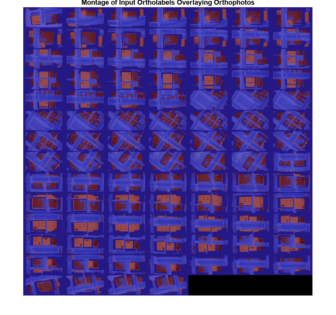

Perform Feature-Based Stitching

Register Orthophoto Pairs

To create the orthomosaic, start by registering successive image pairs using these steps:

Here, $$I(n)$$ is the ${\mathit{n}}^{\mathrm{th}}$ orhophoto from the set of orthophotos in the montage. The Background section provides some visual references for this procedure.

Use the detectKAZEFeatures (Computer Vision Toolbox) function to find the matching features between each orthophoto pair. For more information about the different types of feature detectors and their qualities, see Local Feature Detection and Extraction (Computer Vision Toolbox).

For this detector, set the confidence value to 99.9. Higher confidence values result in slower processing speed, but produce more accurate transforms. You can use a high value for the maximum number of trials to further improve the accuracy of the transforms. Set the maximum number of trials to 2000.

confidenceValue = 99.9;
maxNumTrials = 2000;

Detect Matching Features and Estimate Transforms

Set the random number generator seed to ensure consistency with the example outputs.

rng(250,"twister");

Read the first image from the orthophoto set and initialize the features for the first image by converting it to a grayscale orthophoto.

I = readimage(imdsImg,1);
grayImage = im2gray(I);

Detect and extract the features from the orthophoto.

points = detectKAZEFeatures(grayImage);
[features,points] = extractFeatures(grayImage,points);

Initialize the transformations for all the images as 2-D affine identity matrices.

clear tforms;
numImages = numel(imdsImg.Files);
tforms(numImages) = affine2d(eye(3));

Initialize a variable to hold image sizes.

imageSize = zeros(numImages,2);
imageSize(1,:) = size(grayImage);

For each image, read and convert the image to grayscale and detect its features. Match the points of the features between consecutive orthophotos and use those points to determine the geometric transformation matrices for each pair of orthophotos.

% Show progress bar
f = waitbar(0,"Please wait while transformation matrices are being computed ...",Name="Step [1/5]: Compute transformation matrices");

% Iterate over remaining image pairs
for n = 2:numImages
    
    % Store points and features for I(n-1).
    pointsPrevious = points;
    featuresPrevious = features;
        
    % Read I(n).
    I = readimage(imdsImg, n);
    
    % Convert image to grayscale.
    grayImage = im2gray(I);    
    
    % Save image size.
    imageSize(n,:) = size(grayImage);
    
    % Detect and extract KAZE features for I(n).
    points = detectKAZEFeatures(grayImage);    
    [features,points] = extractFeatures(grayImage,points);
  
    % Find correspondences between I(n) and I(n-1).
    indexPairs = matchFeatures(features,featuresPrevious,Unique=true);
    
    % Get matching points
    matchedPoints = points(indexPairs(:,1), :);
    matchedPointsPrev = pointsPrevious(indexPairs(:,2),:);        
    
    % Estimate the transformation between I(n) and I(n-1).
    tforms(n) = estimateGeometricTransform2D(matchedPoints,matchedPointsPrev, ...
        "affine",Confidence=confidenceValue,MaxNumTrials=maxNumTrials);
    
    % Compute T(n) * T(n-1) * ... * T(1)
    tforms(n).T = tforms(n).T * tforms(n-1).T;

    % Update the progress bar
    progress = n/numImages;
    waitbar(progress,f,sprintf('Finding affine transform matrix for frame number [%d/%d] - %.2f%% Complete\n',n,numImages,progress*100));
end

% Close progress bar
close(f);

Find Central Image

All of the transformations in tforms are relative to the first image. This is a convenient way to perform the image registration procedure because it enables sequential processing of all the images. However, using the first image as the start of the orthomosaic can produce a less accurate orthomosaic because it can distort most of the images that form the orthomosaic. To improve the accuracy of the orthomosaic, modify the transformations so that the center of the scene is the least distorted orthophoto. To accomplish this, invert the transform for the center image and apply that transform to all the other transforms.

First, find the output limits for each transform. Then, use the output limits to automatically find the image that is approximately in the center of the scene.

Compute the output limits for each transform.

xlim = zeros(numel(tforms),2); 
ylim = zeros(numel(tforms),2);
for i = 1:numel(tforms)           
    [currXLim, currYLim] = outputLimits(tforms(i),[1 imageSize(i,2)],[1 imageSize(i,1)]);
    xlim(i,:) = currXLim;
    ylim(i,:) = currYLim;
end

Next, compute the average x-limits and y-limits for each transform, and find the image that is in the center.

avgXLim = mean(xlim,2);
avgYLim = mean(ylim,2);
avgLims = [avgXLim avgYLim];
[~,idx1] = sort(avgLims(:,1));
[~,idx2] = sort(avgLims(idx1,2));
idx = idx1(idx2);
centerIdx = floor((numel(tforms)+1)/2);
centerImageIdx = idx(centerIdx);

Apply Inverse Transform of Central Image

Finally, apply the inverse transform of the center image to all the other transforms.

Tinv = invert(tforms(centerImageIdx));
for i = 1:numel(tforms)    
    tforms(i).T = tforms(i).T * Tinv.T;
end

Initialize the Orthomosaic

To initialize the orthomosaic, you must determine the spatial limits of the orthomosaic. To do so, you must compute the minimum and maximum output limits over all transformations. These values help you compute the size of the final orthomosaic.

Compute the output limits of each transformed image.

for i = 1:numel(tforms)           
    [xlim(i,:), ylim(i,:)] = outputLimits(tforms(i),[1 imageSize(i,2)],[1 imageSize(i,1)]);
end

Find the minimum and maximum output limits values across all transformed orthophotos.

xMin = min(xlim(:));
xMax = max(xlim(:));
yMin = min(ylim(:));
yMax = max(ylim(:));

Calculate and round the xy-ranges to determine the width and height of the final orthomosaic.

width  = round(xMax-xMin);
height = round(yMax-yMin);

Create empty arrays with the computed width and height, one for the orthophoto images and the other for the ortholabels.

orthomosaicImages = zeros([height width 3],like=I);
orthomosaicLabels = zeros([height width 1],like=I);

Compute the Transformed Orthophotos and Ortholabels

You must transform the orthophotos so that you can place them into the orthomosaic.

Use the imwarp function to map images into the orthomosaic, and a vision.AlphaBlender object to overlay the images together. Output the transformed orthoimages, transformed ortholabels, and stitched maps into these folders:

Create a 2-D spatial reference object defining the size of the orthomosaic.

xLimits = [xMin xMax];
yLimits = [yMin yMax];
orthomosaicView = imref2d([height width],xLimits,yLimits);

Initialize variables to hold the images, the labels, and their file paths. Use these to create montages.

warpedImages = cell(1,numImages);
warpedImagePaths = cell(1,numImages);
warpedLabels = cell(1,numImages);
warpedLabelPaths = cell(1,numImages);

Create an output folder to save the transformed images warpedOutputImages.

warpedOutputImageFolderPath = "warpedOutputImages";
exampleHelperMakeFolder(warpedOutputImageFolderPath);

Create an output folder to save the transformed labels warpedOutputLabels.

warpedOutputLabelFolderPath = "warpedOutputLabels";
exampleHelperMakeFolder(warpedOutputLabelFolderPath);

Compute the transformed image and transformed label for each image-label pair using your estimated transformation matrices.

% Show progress bar
f = waitbar(0,"Please wait while the transformed orthophotos are being computed ...",Name="Step [2/5]: Compute transformed orthophotos");

% Compute the warped images and warped labels using the transformation matrices
% obtained earlier
for i = 1:numImages
    
    % Read current image
    I = readimage(imdsImg, i);

    % Obtain its segmap
    C = readimage(imdsLbl, i);
   
    % Transform I into the orthomosaic view.
    warpedImage = imwarp(I, tforms(i), OutputView=orthomosaicView);
    warpedImages{i} = warpedImage;
        
    % Obtain warped label
    warpedLabel = imwarp(C, tforms(i), OutputView=orthomosaicView);
    warpedLabels{i} = warpedLabel;

    % Get the name of the current image
    [~,name,~] = fileparts(imdsImg.Files{i});

    % Save warped image
    warpedImagePath = fullfile(warpedOutputImageFolderPath,sprintf("%s_warped.png",name));
    warpedImagePaths{i} = warpedImagePath;
    imwrite(warpedImage,warpedImagePath);

    % Save warped labels
    warpedLabelPath = fullfile(warpedOutputLabelFolderPath,sprintf("%s_warped.png",name));
    warpedLabelPaths{i} = warpedLabelPath;
    imwrite(warpedLabel,warpedLabelPath);

    % Update the progress bar
    progress = i/numImages;
    waitbar(progress,f,sprintf('Compute the transformed orthophoto for frame number [%d/%d] - %.2f%% Complete\n',i,numImages,progress*100));
end

% Close progress bar
close(f);

Show a montage of the saved transformed images.

warpedOrthophotoMontage = double(montage(warpedImagePaths).CData);
title("Montage of Transformed Orthophotos");

Obtain a montage of the saved transformed labels.

figure("Visible","off");
warpedOrtholabelMontage = montage(warpedLabelPaths,cmap).CData;

Show a montage of the transformed ortholabels overlaid on the transformed orthophotos. Compute the montage ortholabel overlay.

warpedOrthosOverlaid = transparency*warpedOrthophotoMontage/255 + (1-transparency)*warpedOrtholabelMontage;

Show the overlaid montage.

figure;
imshow(warpedOrthosOverlaid);
title("Montage of Transformed Ortholabels Overlaying Transformed Orthophotos");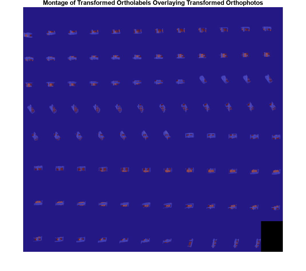

Create and Save Orthomosaic

This example uses the same algorithm to create the orthomosaic as in the Create Panorama (Computer Vision Toolbox) example. However, that example stitches ground-level perspective images, rather than orthographic images, so the algorithm assumes that all pixels in the transformed images have colors (or content). This is not necessarily true for orthographic transformed images, which may have missing regions. As a result, using that algorithm for this application without modification leads to missing pixels in the stitched image. The results from the algorithm would be correct if the transformation matrices you used were perfect, but this is not possible when using automatic marking point and transformation matrix computation.

To prevent missing areas, you can simplify algorithm. While merging images 1 and 2, specify for the algorithm to use the color from whichever image has a color for the current pixel location for that pixel. If both images have colors at that location, such as in the overlap region, perform a blend between the two colors. Set this blend value using the blendFactor variable. A default value of 1 ensures that image 2 completely overwrites image 1 in areas of overlap.

Create and save the outputs of the stitching algorithm for the transformed orthophotos.

Specify the blend factor for common overlapping pixels.

Note that this is the value for the 2nd image. A value of 1 indicates the entire value will be taken from the 2nd image, while 0 means it will be taken from the 1st image.

blendFactor = 1;

Now, stitch the warped images together one by one sequentially.

% Obtain the 1st warped image and its warped labels
I1 = warpedImages{1};
L1 = warpedLabels{1};

% Show progress bar
f = waitbar(0,"Please wait while the transformed orthophotos are being stitched ...",Name="Step [3/5]: Feature-stitch orthophotos");

% Stitch images (and their labels) one by one
for idx = 2:numImages
    
    % Get next image (and its label) in the dataset
    I2 = warpedImages{idx};
    L2 = warpedLabels{idx};

    % Find where I1 has no color
    maskNoColorI1 = I1(:,:,1)==0 & I1(:,:,2)==0 & I1(:,:,3)==0;

    % Find where I2 has no color
    maskNoColorI2 = I2(:,:,1)==0 & I2(:,:,2)==0 & I2(:,:,3)==0;

    % Create mask to take I2's region when I1's region has no color
    mask = maskNoColorI1;

    % Blend the colors of I1 and I2 in regions where they both have color
    % Note: Blend is only taken for image and not for labels as labels are
    % always integer values. Image colors on the other hand can be
    % floating-point values.
    maskImg = mask + (~maskNoColorI1 & ~maskNoColorI2)*blendFactor;
    maskLabels = mask + ~maskNoColorI1 & ~maskNoColorI2;

    % Stitch image
    featureStitchedImg = imblend(I2,I1,imbinarize(maskImg));
    
    % Stitch labels
    featureStitchedLabels = imblend(L2,L1,maskLabels,foregroundopacity=1);

    % Make I1 the stitched image
    I1 = featureStitchedImg;

    % Make L1 the stiched labels
    L1 = featureStitchedLabels;

    % Update the progress bar
    progress = idx/numImages;
    waitbar(progress,f,sprintf('Stitched transformed orthophoto number [%d/%d] - %.2f%% Complete\n',idx,numImages,progress*100));
end

% Close progress bar
close(f);

Show the stitched orthomosaic.

figure;
imshow(featureStitchedImg/255);
title("Stitched Orthomosaic");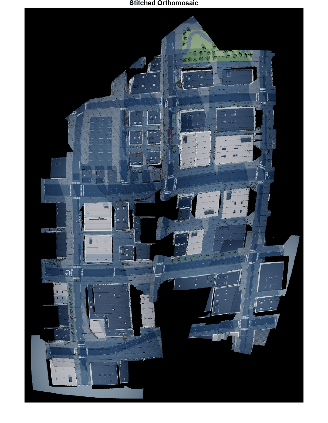

Show the stitched labels overlaying stitched orthomosaic using a colormap.

featureStitchedOverlaid = labeloverlay(featureStitchedImg/255,categorical(featureStitchedLabels),Colormap=cmap,Transparency=transparency);
figure;
imshow(featureStitchedOverlaid);
title("Stitched Orthomosaic - Labels Overlaid");
exampleHelperPixelLabelColorbar(cmap, classNames);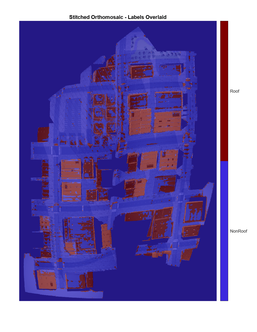

If an output folder for stitched images does not already exist, create one.

stitchedOutputFolderPath = "stitchedOutput";
exampleHelperMakeFolder(stitchedOutputFolderPath);

Save the stitched orthomosaic, stitched labels, and labels overlaid on the stitched orthomosaic as images.

imwrite(featureStitchedImg/255,fullfile(stitchedOutputFolderPath,"featureStitchedOrthophoto.png"));
imwrite(featureStitchedLabels,fullfile(stitchedOutputFolderPath,"featureStitchedOrtholabel.png"));
imwrite(featureStitchedOverlaid,fullfile(stitchedOutputFolderPath,"featureStitchedOrthosOverlaid.png"));

Perform Location-Based Stitching

In the orthomosaic generated from the UAV flying over the US City Block scene, you might notice stitch artifacts due to the feature-based stitching not being as accurate as manual stitching. These errors, caused by incorrect feature-matches, are cumulative, which can cause incorrect stitches for long flight trajectories. Notice that due to the sole dependence on feature-matches, feature-based stitching does not provide any information about the orientation or the scale of the stitched image, which can be arbitrary.

In this section we will look at location-based stitching. Although also prone to accumulation of errors, location-based stitching is more robust as in addition to the data we have seen so far, it also requires the drone's camera roll and camera location for stitching. For more information on why this is the roll and not the yaw of the camera, refer to the Survey Urban Environment Using UAV section of the Survey Urban Environment Using UAV example.

Load Roll and Location Acquired by UAV Flight

Load the flightData MAT file, which contains this data, into the workspace:

H and W are the height and width, respectively, of the acquired images, in pixels. $\mathit{F}$ is the total number of time steps logged and is directly proportional to the flight time.

If indicated that you ran the Survey Urban Environment Using UAV example, a dialog box opens and prompts you to select the path to the flightData.mat file generated by that example.

if strcmp(ranSurveyEx,"true")
    [file,path] = uigetfile("flightData.mat","Select flightData.mat file to open",MultiSelect="off");
    load([path file]);
else
    preAcquiredFlightData = fullfile(preAcquiredDataFolder,"flightData.mat");
    load(preAcquiredFlightData);
end
liveUAVRoll = squeeze(liveUAVRoll);
liveUAVLocation = squeeze(liveUAVLocation);

Determine Roll and Location in World Frame

Loaded liveUAVRoll is in radians. Convert it into degrees.

roll = rad2deg(liveUAVRoll);

liveUAVRoll is still in the local frame of the drone. Convert it into the global frame of Unreal by adding the initial roll of 270 degrees of the drone with respect to the Unreal global frame. This value was determined based on the start orientation of the drone, specified in the Survey Urban Environment Using UAV helper file when the data was captured using the Survey Urban Environment Using UAV example.

roll = 270 + roll;

liveUAVLocation is already in the global frame of Unreal. Hence no changes are needed.

location = liveUAVLocation;

Compute the Rotated Orthophotos and Ortholabels

You must rotate the orthophotos so that you can place them into the orthomosaic.

Use the imrotate function to rotate images for the orthomosaic. Output the rotated orthophotos and ortholabels into these folders:

Initialize variables to hold the images, the labels, and their file paths. Use these to create montages.

rotatedImages = cell(1,numImages);
rotatedImagePaths = cell(1,numImages);
rotatedLabels = cell(1,numImages);
rotatedLabelPaths = cell(1,numImages);

Create an output folder to save the rotated images rotatedOutputImages.

rotatedOutputImageFolderPath = "rotatedOutputImages";
exampleHelperMakeFolder(rotatedOutputImageFolderPath);

Create an output folder to save the rotated labels rotatedOutputLabels.

rotatedOutputLabelFolderPath = "rotatedOutputLabels";
exampleHelperMakeFolder(rotatedOutputLabelFolderPath);

Compute the rotated image and rotated label for each image-label pair using the logged roll.

% Show progress bar
f = waitbar(0,"Please wait while the rotated orthophotos are being computed ...",Name="Step [4/5]: Compute rotated orthophotos");

% Reset orthophoto datastore object
reset(imdsImg);

% Reset ortholabel datastore object
reset(imdsLbl);

% Compute the rotated images and rotated labels using the roll obtained earlier
for i = 1:numImages
    
    % Read current image
    I = readimage(imdsImg, i);

    % Obtain its segmap
    C = readimage(imdsLbl, i);

    % Rotate I into the orthomosaic view
    rotatedImage = imrotate(I,roll(i),"nearest");
    rotatedImages{i} = rotatedImage;

    % Rotate C into the orthomosaic view
    rotatedLabel = imrotate(C,roll(i),"nearest");
    rotatedLabels{i} = rotatedLabel;

    % Get the name of the current image
    [~,name,~] = fileparts(imdsImg.Files{i});

    % Save rotated image
    rotatedImagePath = fullfile(rotatedOutputImageFolderPath,sprintf("%s_rotated.png",name));
    rotatedImagePaths{i} = rotatedImagePath;
    imwrite(rotatedImage,rotatedImagePath);

    % Save rotated labels
    rotatedLabelPath = fullfile(rotatedOutputLabelFolderPath,sprintf("%s_rotated.png",name));
    rotatedLabelPaths{i} = rotatedLabelPath;
    imwrite(rotatedLabel,rotatedLabelPath);

    % Update the progress bar
    progress = i/numImages;
    waitbar(progress,f,sprintf('Computing the rotated orthophoto and ortholabel for frame number [%d/%d] - %.2f%% Complete\n',i,numImages,progress*100));
end

% Close progress bar
close(f);

Show a montage of the saved rotated images.

rotatedOrthophotoMontage = double(montage(rotatedImagePaths).CData);
title("Montage of Rotated Orthophotos");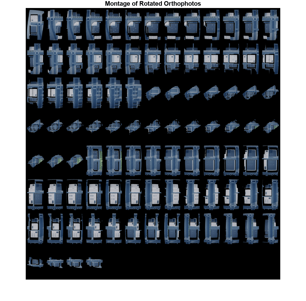

Obtain a montage of the saved rotated labels.

figure("Visible","off");
rotatedOrtholabelMontage = montage(rotatedLabelPaths,cmap).CData;

Show a montage of the rotated ortholabels overlaid on the rotated orthophotos. Compute the montage ortholabel overlay.

rotatedOrthosOverlaid = transparency*rotatedOrthophotoMontage/255 + (1-transparency)*rotatedOrtholabelMontage;

Show the overlaid montage.

figure;
imshow(rotatedOrthosOverlaid);
title("Montage of Rotated Ortholabels Overlaying Rotated Orthophotos");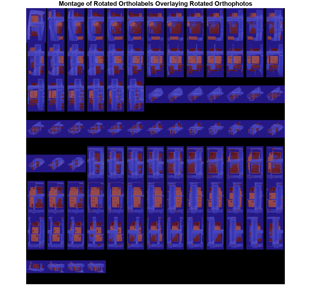

Create and Save Orthomosaic

To create the orthomosaic, start by registering successive image pairs using these steps:

Then take the next consecutive image $$I(n-2)$$, its center point $$P(n-2)$$, stitched image $$I^{\prime }$$, stitched center point $$P^{\prime }$$and repeat the process until all images are exhausted.

Here, $$I(n)$$ is the ${\mathit{n}}^{\mathrm{th}}$ orhophoto from the set of orthophotos in the montage. The Background section provides some visual references for this procedure.

To prevent missing areas, you can simplify algorithm. While merging images 1 and 2, specify for the algorithm to use the color from whichever image has a color for the current pixel location for that pixel. If both images have colors at that location, such as in the overlap region, perform a blend between the two colors. Set this blend value using the blendFactor variable. A default value of 1 ensures that image 2 completely overwrites image 1 in areas of overlap.

Create and save the outputs of the stitching algorithm for the rotated orthophotos.

Specify the blend factor for common overlapping pixels.

Note that this is the value for the 2nd image. A value of 1 indicates the entire value will be taken from the 2nd image, while 0 means it will be taken from the 1st image.

blendFactor = 0;

Now, stitch the rotated images together one by one sequentially.

% Obtain the 1st rotated image and its rotated labels
I1 = rotatedImages{1};

% Get center point for the 1st image
center1 = location(1:2,1);

% Show progress bar
f = waitbar(0,"Please wait while the transformed orthophotos are being stitched ...",Name="Step [5/5]: Location-stitch orthophotos");

% Stitch images (and their labels) one by one
for idx = 2:numImages

    % Get next image (and its label) in the dataset
    I2 = rotatedImages{idx};

    % Get center point for the next image
    center2 = location(1:2,idx);

    % Get corner points for both images
    [topL1,topR1,bottomR1,bottomL1] = exampleHelperComputeImageCornerPoints(I1,center1,meterToPixel,reductionFactor);
    [topL2,topR2,bottomR2,bottomL2] = exampleHelperComputeImageCornerPoints(I2,center2,meterToPixel,reductionFactor);

    % Get X and Y range of stitched output image
    allCorners = [topL1;topR1;bottomL1;bottomR1;topL2;topR2;bottomL2;bottomR2];
    rangeX(1) = min(allCorners(:,1),[],"all");
    rangeX(2) = max(allCorners(:,1),[],"all");
    rangeY(1) = min(allCorners(:,2),[],"all");
    rangeY(2) = max(allCorners(:,2),[],"all");

    % Compute padding needed for images and labels
    [pad1.lPad,pad1.rPad,pad1.tPad,pad1.bPad] = exampleHelperComputeImagePadding(I1,center1,rangeX,rangeY,meterToPixel,reductionFactor);
    [pad2.lPad,pad2.rPad,pad2.tPad,pad2.bPad] = exampleHelperComputeImagePadding(I2,center2,rangeX,rangeY,meterToPixel,reductionFactor);

    % Sync padding to ensure matching padded image sizes
    [pad1,pad2] = exampleHelperSyncImagePadding(I1,pad1,I2,pad2);

    % Add padding to images
    paddedI1 = padarray(I1,double([pad1.tPad pad1.lPad]),'pre');
    paddedI1 = padarray(paddedI1,double([pad1.bPad pad1.rPad]),'post');
    paddedI2 = padarray(I2,double([pad2.tPad pad2.lPad]),'pre');
    paddedI2 = padarray(paddedI2,double([pad2.bPad pad2.rPad]),'post');
    
    % Find where I1 has no color
    maskNoColorI1 = paddedI1(:,:,1)==0 & paddedI1(:,:,2)==0 & paddedI1(:,:,3)==0;
    
    % Find where I2 has no color
    maskNoColorI2 = paddedI2(:,:,1)==0 & paddedI2(:,:,2)==0 & paddedI2(:,:,3)==0;
    
    % Create mask to take I2's region when I1's region has no color
    mask = maskNoColorI1;
    
    % Blend the colors of I1 and I2 in regions where they both have color
    maskImg = mask + (~maskNoColorI1 & ~maskNoColorI2)*blendFactor;
    
    % Stitch image
    locationStitchedImg = imblend(paddedI2,paddedI1,imbinarize(maskImg),foregroundopacity=1);

    % Compute center of stitched image
    stitchedCenter = [sum(rangeX)/2.0 sum(rangeY)/2.0];

    % Make I1 the stitched image
    I1 = locationStitchedImg;

    % Make center1 the stitched center
    center1 = stitchedCenter;

    % Update the progress bar
    progress = idx/numImages;
    waitbar(progress,f,sprintf('Stitched rotated orthophoto number [%d/%d] - %.2f%% Complete',idx,numImages,progress*100));
end

% Close progress bar
close(f);

Show the stitched orthomosaic.

figure;
imshow(locationStitchedImg/255);
title("Stitched Orthomosaic");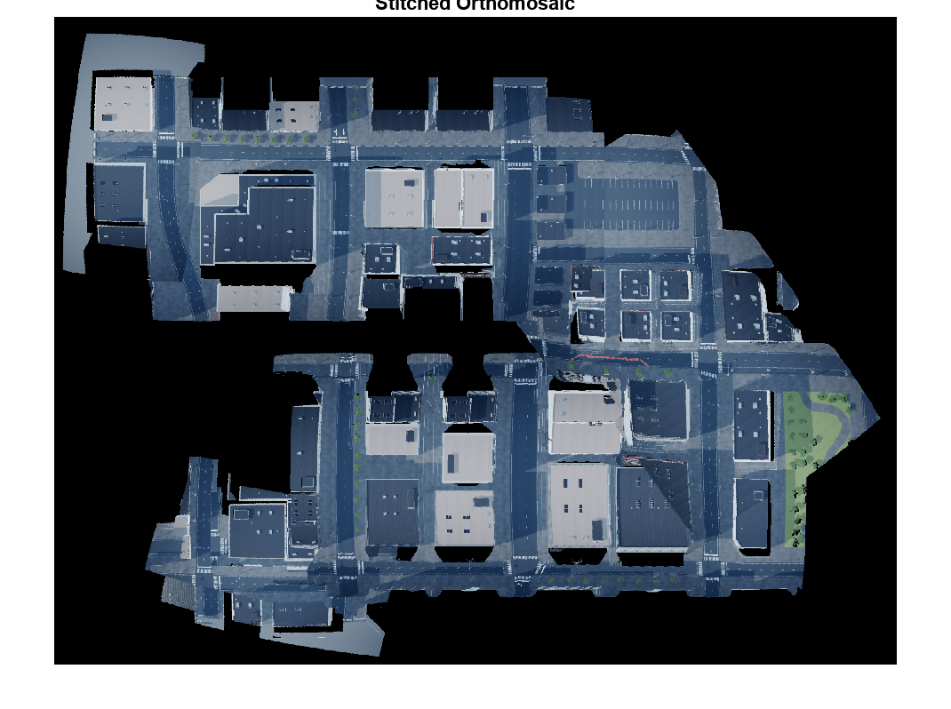

Save the stitched orthomosaic as an image.

imwrite(locationStitchedImg/255,fullfile(stitchedOutputFolderPath,"locationStitchedOrthophoto.png"));

Obtain and Save Labels for Orthomosaic

Load the deep learning network, downloaded in the Setup section, into the workspace.

pretrainedNetwork = fullfile(pretrainedNetworkFolder,"pretrainedNetwork.mat");  
load(pretrainedNetwork);

Obtain labels for the orthomosaic by using the pretrained network.

locationStitchedLabelsCat = semanticseg(locationStitchedImg, net);

Convert the ortholabel from a categorical matrix to a numeric matrix.

locationStitchedLabelsNum = exampleHelperCategoricalToClassIndex(locationStitchedLabelsCat,classNames,classIndexes);

Show the final stitched orthomosaic representing the map of the city.

figure
locationStitchedOverlaid = labeloverlay(locationStitchedImg/255,locationStitchedLabelsCat,Colormap=cmap,Transparency=transparency);
imshow(locationStitchedOverlaid)
title("Orthomosaic - Labels Overlaid")
exampleHelperPixelLabelColorbar(cmap, classNames);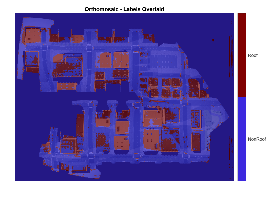

Save the stitched labels, and labels overlaid on the stitched orthomosaic as images.

imwrite(locationStitchedLabelsNum,fullfile(stitchedOutputFolderPath,"locationStitchedOrtholabel.png"));
imwrite(locationStitchedOverlaid,fullfile(stitchedOutputFolderPath,"locationStitchedOrthosOverlaid.png"));

Conclusion

This example showed you how to automatically create an orthomosaic using feature-based and location-based image registration techniques. As a next step, you can use selective image smoothing [1] to deal with stitch artifacts. You can also incorporate additional techniques into the process in this example to improve the blending and alignment of the orthophoto images [2]. Sensor fusion techniques can be used to make the map more accurate by combining the feature-based and location-based stitching techniques, to reduce the accumulation of errors while transforming and stitching.

From a use-case standpoint, you can now use the generated urban city map for numerous applications.

References

[1] Alvarez L, Lions PL, Morel JM. Image Selective Smoothing and Edge Detection by Nonlinear Diffusion. II. SIAM Journal on Numerical Analysis. 1992;29(3):845–866

[2] Matthew Brown and David G. Lowe. 2007. Automatic Panoramic Image Stitching using Invariant Features. Int. J. Compute. Vision 74, 1 (August 2007), 59-73.