Detect Image Anomalies Using Explainable FCDD Network
This example shows how to detect defects on pill images using a one-class fully convolutional data description (FCDD) anomaly detection network.
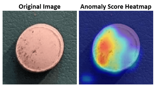
A crucial goal of anomaly detection is for a human observer to be able to understand why a trained network classifies images as anomalies. FCDD enables explainable classification, which supplements the class prediction with information that justifies how the neural network reached its classification decision [1]. The FCDD network returns a heatmap with the probability that each pixel is anomalous. The classifier labels images as normal or anomalous based on the mean value of the anomaly score heatmap.
Download Pill Images for Classification Data Set
This example uses the PillQC data set. The data set contains images from three classes: normal images without defects, chip images with chip defects in the pills, and dirt images with dirt contamination. The data set provides 149 normal images, 43 chip images, and 138 dirt images. The size of the data set is 3.57 MB.
Set dataDir as the desired location of the data set. Download the data set using the downloadPillQCData helper function. This function is attached to the example as a supporting file. The function downloads a ZIP file and extracts the data into the subdirectories chip, dirt, and normal.
dataDir = fullfile(tempdir,"PillDefects");
downloadPillQCData(dataDir)
This image shows an example image from each class. A normal pill with no defects is on the left, a pill contaminated with dirt is in the middle, and a pill with a chip defect is on the right. While the images in this data set contain instances of shadows, focus blurring, and background color variation, the approach used in this example is robust to these image acquisition artifacts.

Load and Preprocess Data
Create an imageDatastore that reads and manages the image data. Label each image as chip, dirt, or normal according to the name of its directory.
imageDir = fullfile(dataDir,"pillQC-main","images");
imds = imageDatastore(imageDir,IncludeSubfolders=true,LabelSource="foldernames");
Partition Data into Training, Calibration, and Test Sets
Create training, calibration, and test sets using the splitAnomalyData function. This example implements an FCDD approach that uses outlier exposure, in which the training data consists primarily of normal images with the addition of a small number of anomalous images. Despite training primarily on samples only of normal scenes, the model learns how to distinguish between normal and anomalous scenes.
Allocate 50% of the normal images and a small percentage (5%) of each anomaly class in the training data set. Allocate 10% of the normal images and 20% of each anomaly class to the calibration set. Allocate the remaining images to the test set.
normalTrainRatio  = 0.5;
anomalyTrainRatio = 0.05;
normalCalRatio  = 0.10;
anomalyCalRatio = 0.20;
normalTestRatio  = 1 - (normalTrainRatio + normalCalRatio);
anomalyTestRatio = 1 - (anomalyTrainRatio + anomalyCalRatio);

anomalyClasses = ["chip","dirt"];
[imdsTrain,imdsCal,imdsTest] = splitAnomalyData(imds,anomalyClasses, ...
    NormalLabelsRatio=[normalTrainRatio normalCalRatio normalTestRatio], ...
    AnomalyLabelsRatio=[anomalyTrainRatio anomalyCalRatio anomalyTestRatio]);
Splitting anomaly dataset
-------------------------
* Finalizing... Done.
* Number of files and proportions per class in all the datasets:

                     Input                  Train                Validation                Test
              NumFiles     Ratio     NumFiles     Ratio      NumFiles     Ratio     NumFiles     Ratio
              ___________________    ____________________    ___________________    ___________________

    chip         43        0.1303        2        0.02381        9       0.17647       32        0.1641
    dirt        138       0.41818        7       0.083333       28       0.54902      103       0.52821
    normal      149       0.45152       75        0.89286       14       0.27451       60       0.30769
Further split the training data into two datastores, one containing only normal data and another containing only anomaly data.
[imdsNormalTrain,imdsAnomalyTrain] = splitAnomalyData(imdsTrain,anomalyClasses, ...
    NormalLabelsRatio=[1 0 0],AnomalyLabelsRatio=[0 1 0],Verbose=false);
Augment Training Data
Augment the training data by using the transform function with custom preprocessing operations specified by the helper function augmentDataForPillAnomalyDetector. The helper function is attached to the example as supporting files.
The augmentDataForPillAnomalyDetector function randomly applies 90 degree rotation and horizontal and vertical reflection to each input image.
imdsNormalTrain = transform(imdsNormalTrain,@augmentDataForPillAnomalyDetector);
imdsAnomalyTrain = transform(imdsAnomalyTrain,@augmentDataForPillAnomalyDetector);
Add binary labels to the calibration and test data sets by using the transform function with the operations specified by the addLabelData helper function. The helper function is defined at the end of this example, and assigns images in the normal class a binary label 0 and images in the chip or dirt classes a binary label 1.
dsCal = transform(imdsCal,@addLabelData,IncludeInfo=true);
dsTest = transform(imdsTest,@addLabelData,IncludeInfo=true);
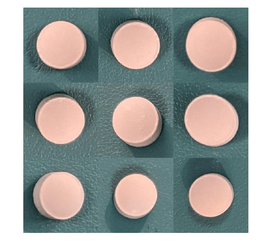
Visualize a sample of nine augmented training images.
exampleData = readall(subset(imdsNormalTrain,1:9));
montage(exampleData(:,1));
Create FCDD Model
This example uses a fully convolutional data description (FCDD) model [1]. The basic idea of FCDD is to train a network to produce an anomaly score map that describes the probability that each region in the input image contains anomaly content.
The pretrainedEncoderNetwork function returns the first three downsampling stages of an ImageNet pretrained Inception-v3 network for use as a pretrained backbone.
backbone = pretrainedEncoderNetwork("inceptionv3",3);Create an FCDD anomaly detector network by using the fcddAnomalyDetector function with the Inception-v3 backbone.
net = fcddAnomalyDetector(backbone);
Train Network or Download Pretrained Network
By default, this example downloads a pretrained version of the FCDD anomaly detector using the helper function downloadTrainedNetwork. The helper function is attached to this example as a supporting file. You can use the pretrained network to run the entire example without waiting for training to complete.
To train the network, set the doTraining variable in the following code to true. Specify the number of epochs to use for training numEpochs by entering a value in the field. Train the model by using the trainFCDDAnomalyDetector function.
Train on one or more GPUs, if available. Using a GPU requires Parallel Computing Toolbox™ and a CUDA® enabled NVIDIA® GPU. For more information, see GPU Computing Requirements (Parallel Computing Toolbox). Training takes about 3 minutes on an NVIDIA Titan RTX™.
doTraining =false; numEpochs =
200; if doTraining options = trainingOptions("adam", ... Shuffle="every-epoch",... MaxEpochs=numEpochs,InitialLearnRate=1e-4, ... MiniBatchSize=32,... BatchNormalizationStatistics="moving"); detector = trainFCDDAnomalyDetector(imdsNormalTrain,imdsAnomalyTrain,net,options); modelDateTime = string(datetime("now",Format="yyyy-MM-dd-HH-mm-ss")); save(fullfile(dataDir,"trainedPillAnomalyDetector-"+modelDateTime+".mat"),"detector"); else trainedPillAnomalyDetectorNet_url = "https://ssd.mathworks.com/supportfiles/"+ ... "vision/data/trainedFCDDPillAnomalyDetectorSpkg.zip"; downloadTrainedNetwork(trainedPillAnomalyDetectorNet_url,dataDir); load(fullfile(dataDir,"folderForSupportFilesInceptionModel", ... "trainedPillFCDDNet.mat")); end
Set Anomaly Threshold
Select an anomaly score threshold for the anomaly detector, which classifies images based on whether their scores are above or below the threshold value. This example uses a calibration data set that contains both normal and anomalous images to select the threshold.
Obtain the mean anomaly score and ground truth label for each image in the calibration set.
scores = predict(detector,dsCal);
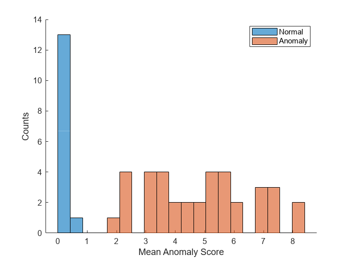
labels = imdsCal.Labels ~= "normal";Plot a histogram of the mean anomaly scores for the normal and anomaly classes. The distributions are well separated by the model-predicted anomaly score.
numBins = 20;
[~,edges] = histcounts(scores,numBins);
figure
hold on
hNormal = histogram(scores(labels==0),edges);
hAnomaly = histogram(scores(labels==1),edges);
hold off
legend([hNormal,hAnomaly],"Normal","Anomaly")
xlabel("Mean Anomaly Score")
ylabel("Counts")
Calculate the optimal anomaly threshold by using the anomalyThreshold function. Specify the first two input arguments as the ground truth labels, labels, and predicted anomaly scores, scores, for the calibration data set. Specify the third input argument as true because true positive anomaly images have a labels value of true. The anomalyThreshold function returns the optimal threshold and the receiver operating characteristic (ROC) curve for the detector, stored as an rocmetrics (Deep Learning Toolbox) object.
[thresh,roc] = anomalyThreshold(labels,scores,true);
Set the Threshold property of the anomaly detector to the optimal value.
detector.Threshold = thresh;
Plot the ROC by using the plot (Deep Learning Toolbox) object function of rocmetrics. The ROC curve illustrates the performance of the classifier for a range of possible threshold values. Each point on the ROC curve represents the false positive rate (x-coordinate) and true positive rate (y-coordinate) when the calibration set images are classified using a different threshold value. The solid blue line represents the ROC curve. The red dashed line represents a no-skill classifier corresponding to a 50% success rate. The ROC area under the curve (AUC) metric indicates classifier performance, and the maximum ROC AUC corresponding to a perfect classifier is 1.0.
plot(roc)
title("ROC AUC: "+ roc.AUC)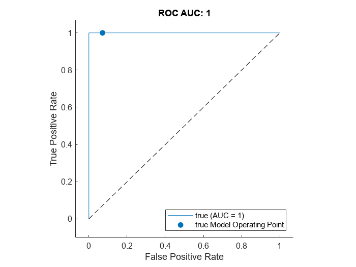
Evaluate Classification Model
Classify each image in the test set as either normal or anomalous.
testSetOutputLabels = classify(detector,dsTest);
Get the ground truth labels of each test image.
testSetTargetLabels = dsTest.UnderlyingDatastores{1}.Labels;Evaluate the anomaly detector by calculating performance metrics by using the evaluateAnomalyDetection function. The function calculates several metrics that evaluate the accuracy, precision, sensitivity, and specificity of the detector for the test data set.
metrics = evaluateAnomalyDetection(testSetOutputLabels,testSetTargetLabels,anomalyClasses);
Evaluating anomaly detection results
------------------------------------
* Finalizing... Done.
* Data set metrics:

    GlobalAccuracy    MeanAccuracy    Precision    Recall     Specificity    F1Score    FalsePositiveRate    FalseNegativeRate
    ______________    ____________    _________    _______    ___________    _______    _________________    _________________

       0.96923          0.97778           1        0.95556         1         0.97727            0                0.044444
The ConfusionMatrix property of metrics contains the confusion matrix for the test set. Extract the confusion matrix and display a confusion plot. The classification model in this example is very accurate and predicts a small percentage of false positives and false negatives.
M = metrics.ConfusionMatrix{:,:};
confusionchart(M,["Normal","Anomaly"])
acc = sum(diag(M)) / sum(M,"all");
title("Accuracy: "+acc)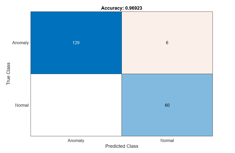
If you specify multiple anomaly class labels, such as dirt and chip in this example, the evaluateAnomalyDetection function calculates metrics for the whole data set and for each anomaly class. The per-class metrics are returned in the ClassMetrics property of the anomalyDetectionMetrics object, metrics.
metrics.ClassMetrics
ans=2×2 table
         1    1×1 table
    0.9556    2×1 table
metrics.ClassMetrics(2,"AccuracyPerSubClass").AccuracyPerSubClass{1}ans=2×1 table
0.8438
0.9903
Explain Classification Decisions
You can use the anomaly heatmap predicted by the anomaly detector to help explain why an image is classified as normal or anomalous. This approach is useful for identifying patterns in false negatives and false positives. You can use these patterns to identify strategies for increasing class balancing of the training data or improving the network performance.
Calculate Anomaly Heat Map Display Range
Calculate a display range that reflects the range of anomaly scores observed across the entire calibration set, including normal and anomalous images. Using the same display range across images allows you to compare images more easily than if you scale each image to its own minimum and maximum. Apply the display range for all heatmaps in this example.
minMapVal = inf;
maxMapVal = -inf;
reset(dsCal)
while hasdata(dsCal)
    img = read(dsCal);
    map = anomalyMap(detector,img{1});
    minMapVal = min(min(map,[],"all"),minMapVal);
    maxMapVal = max(max(map,[],"all"),maxMapVal);
end
displayRange = [minMapVal,maxMapVal];
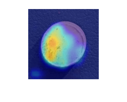
View Heatmap of Anomaly Image
Select an image of a correctly classified anomaly. This result is a true positive classification. Display the image.
testSetAnomalyLabels = testSetTargetLabels ~= "normal";
idxTruePositive = find(testSetAnomalyLabels' & testSetOutputLabels,1,"last");
dsExample = subset(dsTest,idxTruePositive);
img = read(dsExample);
img = img{1};
map = anomalyMap(detector,img);
imshow(anomalyMapOverlay(img,map,MapRange=displayRange,Blend="equal"))
View Heatmap of Normal Image
Select and display an image of a correctly classified normal image. This result is a true negative classification.
idxTrueNegative = find(~(testSetAnomalyLabels' | testSetOutputLabels));
dsExample = subset(dsTest,idxTrueNegative);
img = read(dsExample);
img = img{1};
map = anomalyMap(detector,img);
imshow(anomalyMapOverlay(img,map,MapRange=displayRange,Blend="equal"))
View Heatmaps of False Negative Images
False negatives are images with pill defect anomalies that the network classifies as normal. Use the explanation from the network to gain insights into the misclassifications.
Find any false negative images from the test set. Obtain heatmap overlays of the false negative images by using the transform function. The operations of the transform are specified by an anonymous function that applies the anomalyMapOverlay function to obtain heatmap overlays for each false negative in the test set.
falseNegativeIdx = find(testSetAnomalyLabels' & ~testSetOutputLabels);
if ~isempty(falseNegativeIdx)
    fnExamples = subset(dsTest,falseNegativeIdx);
    fnExamplesWithHeatmapOverlays = transform(fnExamples,@(x) {...
        anomalyMapOverlay(x{1},anomalyMap(detector,x{1}), ...
        MapRange=displayRange,Blend="equal")});
    fnExamples = readall(fnExamples);
    fnExamples = fnExamples(:,1);
    fnExamplesWithHeatmapOverlays = readall(fnExamplesWithHeatmapOverlays);
    montage(fnExamples)
    montage(fnExamplesWithHeatmapOverlays)
else
    disp("No false negatives detected.")
end

View Heatmaps of False Positive Images
False positives are images without pill defect anomalies that the network classifies as anomalous. Find any false positives in the test set. Use the explanation from the network to gain insights into the misclassifications. For example, if anomalous scores are localized to the image background, you can explore suppressing the background during preprocessing.
falsePositiveIdx = find(~testSetAnomalyLabels' & testSetOutputLabels);
if ~isempty(falsePositiveIdx)
    fpExamples = subset(dsTest,falsePositiveIdx);
    fpExamplesWithHeatmapOverlays = transform(fpExamples,@(x) { ...
        anomalyMapOverlay(x{1},anomalyMap(detector,x{1}), ...
        MapRange=displayRange,Blend="equal")});
    fpExamples = readall(fpExamples);
    fpExamples = fpExamples(:,1);
    fpExamplesWithHeatmapOverlays = readall(fpExamplesWithHeatmapOverlays);
    montage(fpExamples)
    montage(fpExamplesWithHeatmapOverlays)
else
    disp("No false positives detected.")
end
No false positives detected.
Supporting Functions
The addLabelData helper function creates a one-hot encoded representation of label information in data.
function [data,info] = addLabelData(data,info)
    if info.Label == categorical("normal")
        onehotencoding = 0;
    else
        onehotencoding = 1;
    end
    data = {data,onehotencoding};
end
References
[1] Liznerski, Philipp, Lukas Ruff, Robert A. Vandermeulen, Billy Joe Franks, Marius Kloft, and Klaus-Robert Müller. "Explainable Deep One-Class Classification." Preprint, submitted March 18, 2021. https://arxiv.org/abs/2007.01760.
[2] Ruff, Lukas, Robert A. Vandermeulen, Billy Joe Franks, Klaus-Robert Müller, and Marius Kloft. "Rethinking Assumptions in Deep Anomaly Detection." Preprint, submitted May 30, 2020. https://arxiv.org/abs/2006.00339.
[3] Simonyan, Karen, and Andrew Zisserman. "Very Deep Convolutional Networks for Large-Scale Image Recognition." Preprint, submitted April 10, 2015. https://arxiv.org/abs/1409.1556.
[4] ImageNet. https://www.image-net.org.
See Also
transform | pretrainedEncoderNetwork | fcddAnomalyDetector | trainFCDDAnomalyDetector | predict | anomalyThreshold | anomalyMapOverlay | evaluateAnomalyDetection | anomalyDetectionMetrics | rocmetrics (Deep Learning Toolbox) | confusionchart (Deep Learning Toolbox)
Topics
- Detect Anomalies in Pills During Live Image Acquisition (Image Acquisition Toolbox)
- Detect Image Anomalies Using Pretrained ResNet-18 Feature Embeddings
- Classify Defects on Wafer Maps Using Deep Learning
- Getting Started with Anomaly Detection Using Deep Learning
- Datastores for Deep Learning (Deep Learning Toolbox)