Detect Industrial Defects Using Zero-Shot AnomalyCLIP
This example shows how to detect and localize industrial production defects in pill images using an AnomalyCLIP anomaly detection network.
The AnomalyCLIP model is a zero-shot, multi-class anomaly detector constructed using architecture modification and fine-tuning of the CLIP model [1][2]. The CLIP model is trained to embed both text and images into a shared embedding space in which the distance between embeddings indicates similarity. AnomalyCLIP modifies CLIP to learn universal text embeddings for normal and anomalous objects. During inference, the model compares the new image's embedding to the learned embeddings to decide if the image is normal or anomalous. To localize anomalies in an image, AnomalyCLIP uses information from different layers of CLIP to create a global heatmap that highlights the anomalous areas. AnomalyCLIP offers these key advantages:
AnomalyCLIP automatically learns to differentiate between normal and anomalous images, eliminating the explicit need for user-defined textual prompts that traditionally guide other models, setting it apart from previous text-guided anomaly detectors.
The model’s architecture allows for a single flexible deployment across a wide range of object classes. You can use AnomalyCLIP pretrained on one set of object classes to effectively classify new types of images that contain object classes it hasn't seen before, without requiring more training.
In this example, you first load an AnomalyCLIP network pretrained on the VisA data set [3] and then, you perform inference on a different class data set containing industrial images of pills. You set an anomaly threshold, evaluate the model's classification decisions, and inspect the results for correct and incorrect predictions.
Download Pretrained AnomalyCLIP Detector
By default, this example downloads a pretrained version of an AnomalyCLIP anomaly detector using the helper function downloadTrainedNetwork. The function is attached to this example as a supporting file.
trainedAnomalyCLIPNet_url = "https://ssd.mathworks.com/supportfiles/" + ...
     "vision/data/trainedVisADetectorAnomalyCLIP.zip";
downloadTrainedNetwork(trainedAnomalyCLIPNet_url,pwd)
Downloading pretrained network.
This can take several minutes to download...
Done.
Download Pill QC Data Set
Load the PillQC data set of 330 color images (149 normal images and 151 anomalous images) [4]. The images depict pills captured from an orthogonal view. The anomalous images contain defects such as dirt contamination or chips in the pill structure.
Specify dataDir as the location of the data set. Download the data set using the downloadPillQCData helper function. This function, which is attached to the example as a supporting file, downloads a ZIP file and extracts the data.
dataDir = fullfile(tempdir,"PillQC");
downloadPillQCData(dataDir)
Downloading Pill QC data set. This can take several minutes to download and unzip... Done.
Configure AnomalyCLIP Detector
Load the AnomalyCLIP anomaly detector using the anomalyCLIPDetector helper function, which is attached to the example as a supporting file.
detector = anomalyCLIPDetector;
Localize Defects in Sample Images
Read two sample anomalous images with "chip" and "dirt" labels from the data set.
sampleImageChip = imread(fullfile(dataDir,"pillQC-main", ...
    "images","chip","chip0001.jpg"));
sampleImageChip = imresize(sampleImageChip, OutputSize=detector.ImageSize(1:2));
sampleImageDirt = imread(fullfile(dataDir,"pillQC-main", ...
    "images","dirt","dirt0001.jpg"));
sampleImageDirt = imresize(sampleImageDirt, OutputSize=detector.ImageSize(1:2));
Visualize the localization of defects for each sample anomalous image by displaying the original images with the overlaid predicted per-pixel anomaly score map. Use the anomalyMap function to generate the anomaly score heatmap for the sample image. Display the image, with the heatmap overlaid by using the anomalyMapOverlay function.
anomalyHeatMapChip = anomalyMap(detector,sampleImageChip);
heatMapImageChip = anomalyMapOverlay(sampleImageChip,anomalyHeatMapChip);
montage({sampleImageChip,heatMapImageChip})
title("Heatmap of Anomalous Pill with Chip")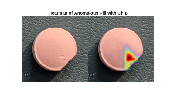
anomalyHeatMapDirt = anomalyMap(detector,sampleImageDirt);
heatMapImageDirt = anomalyMapOverlay(sampleImageDirt,anomalyHeatMapDirt);
montage({sampleImageDirt,heatMapImageDirt})
title("Heatmap of Anomalous Pill with Dirt")
Prepare Data for Evaluation
Create an imageDatastore object that holds the pill image data, and display the defect count based on the image labels.
exts = {".jpg",".png",".tif"};
dsTest = imageDatastore(fullfile(dataDir,"pillQC-main","images"),IncludeSubfolders=true,LabelSource="foldernames");
resizeImage = @(img) imresize(img, detector.ImageSize(1:2));
dsTest.ReadFcn = @(filename) resizeImage(imread(filename));
summary(dsTest.Labels)
330×1 categorical
chip 43
dirt 138
normal 149
<undefined> 0
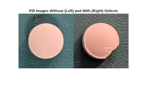
Display images of a normal and defective pills from the test data set.
badImage = find(dsTest.Labels=="chip",1);
badImage = read(subset(dsTest,badImage));
normalImage = find(dsTest.Labels=="normal",1);
normalImage = read(subset(dsTest,normalImage));
montage({normalImage,badImage})
title("Pill Images Without (Left) and With (Right) Defects")
Partition Data into Calibration and Test Sets
Prior to partitioning the data, set the global random state to "default" to ensure reproducibility.
rng("default")Use a calibration set to determine the threshold for the classifier. Using separate calibration and test sets avoids information leaking from the test set into the design of the classifier. The classifier labels images with anomaly scores above the threshold as anomalous.
To establish a suitable threshold for the classifier, allocate 50% of the test data set as the calibration set, which has nearly equal numbers of normal and anomalous images.
[dsCal,dsTest] = splitEachLabel(dsTest,0.5,"randomized");Set Anomaly Threshold
During semi-supervised anomaly detection, you must choose an anomaly score threshold for separating normal images from anomalous images. Select an anomaly score threshold for the anomaly detector, which classifies images based on whether their scores are above or below the threshold value. This example uses the calibration data sets defined in the Partition Data into Calibration and Test Sets section, which contains both normal and anomalous images to select the threshold. Since AnomalyCLIP is a multi-class detector, you can select one anomaly threshold for all classes, or assign a unique anomaly threshold for each class. Since the data set in this example contains a single object class, all images contain the same anomaly threshold.
Compute the maximum anomaly score and ground truth label for each image in the calibration set by using the predict object function. Specify the MiniBatchSize argument value as 4, or another small number to prevent out-of-memory errors.
scoresCal = predict(detector,dsCal,MiniBatchSize=4);
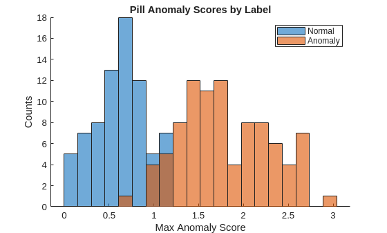
labelsCal = dsCal.Labels~="normal";Plot a histogram of the maximum anomaly scores for the normal and anomalous classes. The figure shows that the distributions are well-separated by the model-predicted anomaly score.
numBins = 20;
figure
[~,edges] = histcounts(scoresCal,numBins);
hold on
hNormal = histogram(scoresCal(labelsCal==0),edges);
hAnomaly = histogram(scoresCal(labelsCal==1),edges);
hold off
legend([hNormal,hAnomaly],"Normal","Anomaly")
xlabel("Max Anomaly Score")
ylabel("Counts")
title("Pill Anomaly Scores by Label")
Calculate the optimal anomaly threshold by using the anomalyThreshold function. Specify the first two input arguments as the data labels, labelsCal, and predicted anomaly scores, scoresCal, for the calibration data set. Specify the third input argument as true because true positive anomaly images have a labels value of true. The anomalyThreshold function returns the optimal threshold value as a scalar and the receiver operating characteristic (ROC) curve for the detector as an rocmetrics (Deep Learning Toolbox) object.
[thresh,roc] = anomalyThreshold(labelsCal,scoresCal,true);
Plot the ROC curve by using the plot (Deep Learning Toolbox) object function of rocmetrics. The ROC curve illustrates the performance of the classifier for a range of possible threshold values. Each point on the ROC curve represents the false positive rate (x-coordinate) and true positive rate (y-coordinate) when you classify the calibration set images using a different threshold value. The solid blue line represents the ROC curve. The area under the ROC curve (AUC) metric indicates classifier performance, with a perfect classifier corresponding to the maximum ROC AUC 1.0.
figure
plot(roc)
title("Pill ROC AUC: " + roc.AUC)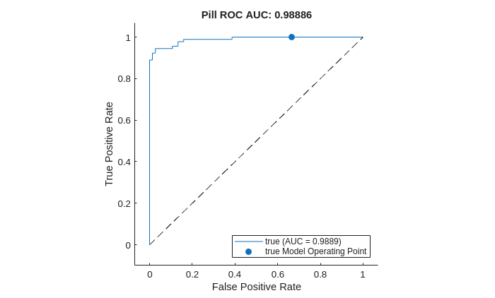
Evaluate Classification Model
Classify each image in the test set as either normal or anomalous by using the classify object function. Specify the MiniBatchSize argument as 4, or another small number to prevent out-of-memory errors. Set the Threshold property of the anomaly detector to the computed optimal threshold value.
detector.Threshold = thresh;
Y = classify(detector,dsTest,MiniBatchSize=4);
Get the ground truth labels of each test image.
gtLabels = dsTest.Labels ~= "normal";Evaluate the anomaly detector by calculating performance metrics using the evaluateAnomalyDetection function. The function calculates several metrics that evaluate the accuracy, precision, sensitivity, and specificity of the detector for the test data set.
metrics = evaluateAnomalyDetection(Y,gtLabels,1);
Evaluating anomaly detection results
------------------------------------
* Finalizing... Done.
* Data set metrics:

    GlobalAccuracy    MeanAccuracy    Precision    Recall     Specificity    F1Score    FalsePositiveRate    FalseNegativeRate
    ______________    ____________    _________    _______    ___________    _______    _________________    _________________

       0.93293          0.93529        0.96471     0.91111      0.95946      0.93714        0.040541             0.088889
The ConfusionMatrix property of metrics contains the confusion matrix for the test set. Extract the confusion matrix and display a confusion plot. The classification model in this example is very accurate and predicts a small percentage of false positives and false negatives.
figure
m = metrics.ConfusionMatrix{:,:};
confusionchart(m,["Normal","Anomaly"])
acc = sum(diag(m))/sum(m,"all");
title("Pill Anomaly Classification Accuracy: " + acc)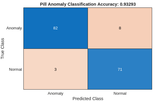
Explain Classification Decisions
You can use the anomaly heatmap that the anomaly detector predicts to explain why the detector classifies an image as normal or anomalous. This approach is useful for identifying patterns in false negatives and false positives.
Normalize Anomaly Heat Map Display Range
To compare anomaly scores observed across the entire calibration set, including normal and anomalous images, normalize the anomaly score map display range. By using the same display range across images, you can compare images more easily than if you scale each image to its own minimum and maximum.
Define a normalized display range, displayRange, that reflects the range of anomaly scores observed across the entire calibration set, including normal and anomalous images for all classes.
minMapVal = inf;
maxMapVal = -inf;
reset(dsCal)
while hasdata(dsCal)
    img = read(dsCal);
    map = anomalyMap(detector,img);
    minMapVal = min(min(map,[],"all"),minMapVal);
    maxMapVal = max(max(map,[],"all"),maxMapVal);
end
displayRange = [minMapVal maxMapVal];
View Heatmaps of Anomalous Images
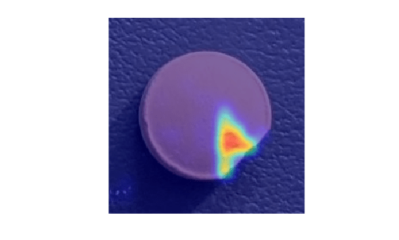
Select images of a correctly classified anomalies for each class. Display the images with the heatmap overlaid using the anomalyMapOverlay function.
idxTruePositive = find(gtLabels & Y);
if ~isempty(idxTruePositive)
    img = readimage(dsTest, idxTruePositive(80));
    map = anomalyMap(detector, img);
    mapOverlay = anomalyMapOverlay(img,map,MapRange=displayRange,Blend="equal");
    figure
    imshow(mapOverlay)
end
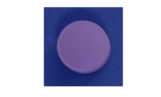
View Heatmaps of Normal Images
Select and display images of correctly classified normal objects, with the heatmap overlaid by using the anomalyMapOverlay function.
idxTrueNegative = find(~(gtLabels | Y));
if ~isempty(idxTrueNegative)
    img = readimage(dsTest, idxTrueNegative(1));
    map = anomalyMap(detector, img);
    mapOverlay = anomalyMapOverlay(img,map,MapRange=displayRange,Blend="equal");
    figure
    imshow(mapOverlay)
end
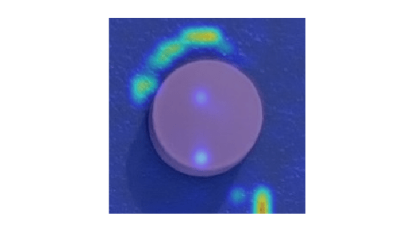
View Heatmaps of False Positive Images
False positives are images without defects that the network misclassifies as anomalous. Use the explanation from the AnomalyCLIP model [1] to gain insight into the misclassifications.
Select a false positive image, and display it, with the heatmap overlaid by using the anomalyMapOverlay function. For this test image, anomalous scores are localized to image areas with uneven lightning, so you might consider adjusting the image contrast during preprocessing, increasing the number of images used for training, or choosing a different threshold at the calibration step.
idxFalsePositive = find(~(gtLabels) & Y);
if ~isempty(idxFalsePositive)
    img = readimage(dsTest, idxFalsePositive(1));
    map = anomalyMap(detector,img);
    figure
    imshow(anomalyMapOverlay(img,map,MapRange=displayRange,Blend="equal"))
end
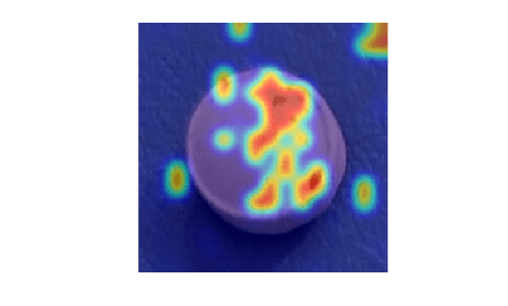
View Heatmap of False Negative Image
False negatives are images with defects, but that the network misclassifies as normal. Use the explanation from the AnomalyCLIP model [1] to gain insight into the misclassifications.
Select a false negative image, and display it, with the heatmap overlaid by using the anomalyMapOverlay function. To decrease false negative results, consider adjusting the anomaly threshold.
idxFalseNegative = find(gtLabels & (~Y));
if ~isempty(idxFalseNegative)
    img = readimage(dsTest, idxFalseNegative(1));
    map = anomalyMap(detector, img);
    figure
    imshow(anomalyMapOverlay(img,map,MapRange=displayRange,Blend="equal"))
end
References
[1] Zhou, Qihang, Guansong Pang, Yu Tian, Shibo He, and Jiming Chen. “AnomalyCLIP: Object-agnostic Prompt Learning for Zero-shot Anomaly Detection.” In The Twelfth International Conference on Learning Representations, 2024. https://doi.org/10.48550/arXiv.2310.18961.
[2] Radford, Alec, Jong Wook Kim, Chris Hallacy, Aditya Ramesh, Gabriel Goh, Sandhini Agarwal, Girish Sastry et al. "Learning transferable visual models from natural language supervision." In International conference on machine learning, pp. 8748-8763. PmLR, 2021. https://doi.org/10.48550/arXiv.2103.00020.
[3] Zou, Yang, Jongheon Jeong, Latha Pemula, Dongqing Zhang, and Onkar Dabeer. "SPot-the-Difference Self-Supervised Pre-Training for Anomaly Detection and Segmentation." arXiv, July 28, 2022. https://doi.org/10.48550/arXiv.2207.14315.
[4] Taylor, Alex. "PillQC: A pill quality control dataset and associated anomaly detection example." GitHub. January 13, 2022. https://github.com/matlab-deep-learning/pillQC.
See Also
anomalyMap | predict | evaluateAnomalyDetection | anomalyThreshold