Detect Defects Using Tiled Training of EfficientAD Anomaly Detector

Download Pretrained EfficientAD Detector

By default, this example downloads a pretrained version of the EfficientAD anomaly detector using the helper function downloadTrainedNetwork. The function is attached to this example as a supporting file. You can use the pretrained network to run the entire example without waiting for training to complete. The fully convolutional architecture of EfficientAD enables tiled training and full-size inference without the need for multiple inference calls per image.

trainedGumDefectDetectorNet_url = "https://ssd.mathworks.com/supportfiles/" + ...
     "vision/data/trainedGumDefectDetectorEfficientAD.zip";
downloadTrainedNetwork(trainedGumDefectDetectorNet_url,pwd)
load("trainedGumDefectDetectorEfficientAD.mat")

Download VisA Data Set

Load the Visual Anomaly (VisA) data set of 10,821 high-resolution color images (9,621 normal and 1,200 anomalous samples) covering 12 different object subsets in 3 domains [2]. Several data subsets contain industrial production images of chewing gum, cashews, fryums, and other food. The anomalous images in the chewing gum test set contain surface defects such as scratches, dents, color spots as well as structural defects such as broken edges.

This example uses the chewing gum data subset. This data subset contains train and test folders, which include the normal training images, and the normal and anomalous test images, respectively.

Specify dataDir as the location of the data set. Download the data set using the downloadVisAData helper function. This function, which is attached to the example as a supporting file, downloads a ZIP file and extracts the data.

dataDir = fullfile(tempdir,"VisA");
downloadVisAData(dataDir)

Localize Defects in Image

Read a sample anomalous image with a "bad" label from the data set.

sampleImage = imread(fullfile(dataDir,"VisA", ...
    "chewinggum","test","bad","000.JPG"));

Visualize the localization of defects by displaying the original chewing gum image with the overlaid predicted per-pixel anomaly score map. Use the anomalyMap function to generate the anomaly score heatmap for the sample image. Display the image, with the heatmap overlaid by using the anomalyMapOverlay function.

anomalyHeatMap = anomalyMap(detector,sampleImage);
heatMapImage = anomalyMapOverlay(sampleImage,anomalyHeatMap);
montage({sampleImage,heatMapImage})
title("Heatmap of Anomalous Image")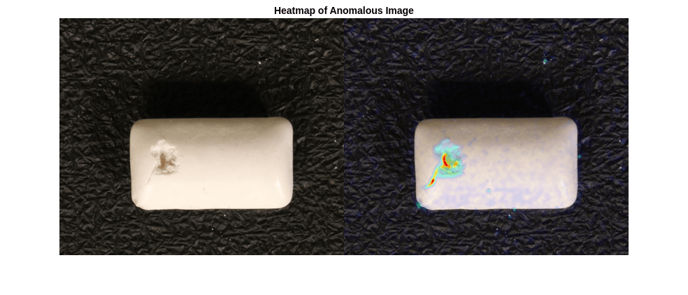

Prepare Data for Training

Create imageDatastore objects that hold the training and test sets, from the train and test folders of the downloaded VisA data set.

exts = {".jpg",".png",".tif"};
dsTrain = imageDatastore(fullfile(dataDir,"VisA","chewinggum","train"),IncludeSubfolders=true,LabelSource="foldernames");
summary(dsTrain.Labels)

453×1 categorical

     good             453 
     <undefined>        0 

normalLabelStr = "good";
dsTest = imageDatastore(fullfile(dataDir,"VisA","chewinggum","test"),IncludeSubfolders=true,LabelSource="foldernames");
summary(dsTest.Labels)

150×1 categorical

     bad              100 
     good              50 
     <undefined>        0 

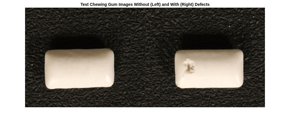
Display images of a normal piece of chewing gum and a defective piece of chewing gum from the test data set.

badImage = find(dsTest.Labels=="bad",1);
badImage = read(subset(dsTest,badImage));
normalImage = find(dsTest.Labels=="good",1);
normalImage = read(subset(dsTest,normalImage));
montage({normalImage,badImage})
title("Test Chewing Gum Images Without (Left) and With (Right) Defects")

Partition Data into Calibration and Test Sets

Prior to partitioning the data, set the global random state to "default" to ensure reproducibility.

rng("default")

Use a calibration set to determine the threshold for the classifier. Using separate calibration and test sets avoids information leaking from the test set into the design of the classifier. The classifier labels images with anomaly scores above the threshold as anomalous.

To establish a suitable threshold for the classifier, allocate 50% of the original test set as the calibration set dsCal, which has equal numbers of normal and anomalous images.

[dsCal,dsTest] = splitEachLabel(dsTest,0.5,"randomized");

Prepare Data For Training

Split Data into Masked Tiles

Create a blockedImage object from the images in the training set. The blockedImage object represents an image as a collection of smaller tiles, or blocks, of size 256-by-256 pixels. For each block, create a logical mask, in which true (or 1) pixels represent regions of interest that contain meaningful normal data, by specifying the maskObjectsInNormalImages helper function handle to the apply function as the processing function input. Save the blocked image masks normalMasks to the location of the mask folder you create trainNormalMaskDir.

trainNormalMaskDir = fullfile(dataDir,"EAD","chewinggum","train",normalLabelStr+"_masks");
blockSize = [256 256];
if ~isfolder(trainNormalMaskDir)
    bims = blockedImage(dsTrain.Files);

    % Find a global threshold from one normal image to segment
    % chewing gum images. Images in this data set are mostly uniformly
    % illuminated so the same threshold can be used for all images.
    im = gather(bims(1));
    T = graythresh(im);

    normalMasks = apply(bims,@(x)maskObjectsInNormalImages(x,T), ...
        BlockSize=blockSize,OutputLocation=trainNormalMaskDir, ...
        Adapter=images.blocked.PNGBlocks,UseParallel=false);

    save(fullfile(trainNormalMaskDir,normalLabelStr+"_masks.mat"),"normalMasks")

else
    load(fullfile(trainNormalMaskDir,normalLabelStr+"_masks.mat"),"normalMasks")
end

Select Training Tiles and Write Data to Disk

To accelerate training speed, create an on-disk representation of the blocked image mask data. Select blocked tiles for training that include a normal image of an object with meaningful data by using the selectBlockLocations function. To help the detector learn the background features also present in anomalous images, specify the InclusionThreshold argument as 0.

Write image tiles to disk using the writeall function, and display sample tiles. If you have a Parallel Computing Toolbox™ license, specify the UseParallel argument as true to reduce processing time.

normalBlocksDir = fullfile(dataDir,"EAD","chewinggum","train",normalLabelStr);
if ~isfolder(normalBlocksDir)
    bims = blockedImage(dsTrain.Files);

    % Select blocks based on the masks computed in the previous step
    bls = selectBlockLocations(bims,Levels=1,BlockSize=blockSize, ...
        Mask=normalMasks,ExcludeIncompleteBlocks=true,BlockOffsets=blockSize, ...
        InclusionThreshold=0,UseParallel=false);
    bimds = blockedImageDatastore(bims,BlockLocationSet=bls);

    % Write all tiles to disk
    writeall(bimds,normalBlocksDir,UseParallel=false)

    % Display a few blocks
    bimds.ReadSize = 10;
    blocks = read(bimds);
    figure
    montage(blocks,BorderSize=5,BackgroundColor="b")
end

Create Training, Test, and Calibration Datastores

Create an ImageDatastore object that contains the training tiles.

dsTrainTiles = imageDatastore(normalBlocksDir,IncludeSubfolders=true,FileExtensions=".png",LabelSource="foldernames");

Add one-hot encoded labels to the training data using the transform function. Specify the transform function using the addLabelData helper function.

dsTrainTiles = transform(dsTrainTiles,@addLabelData,IncludeInfo=true);

Similarly, add one-hot encoded labels to the calibration and test data using the transform function and the addLabelData helper function.

dsCal = transform(dsCal,@addLabelData,IncludeInfo=true);
dsTest = transform(dsTest,@addLabelData,IncludeInfo=true);

Define EfficientAD Object Detector Network Architecture

Create the EfficientAD anomaly detector using the efficientADAnomalyDetector object. Specify the UseGlobalAnomalyMap argument as false to turn off the autoencoder and use only the student-teacher model. This enables the model to generalize learned features from training on image tiles to the full-resolution image at inference time.

untrainedDetector = efficientADAnomalyDetector(Network="pdn-small",UseGlobalAnomalyMap=false);

Specify Training Options and Train Detector

To train the detector, set the doTraining variable to true.

Train the EfficientAD anomaly detector by using the trainEfficientADAnomalyDetector function. Specify the MapNormalizationDataRatio argument as 0.2 to compute percentile normalization statistics for the student model for 20% of the training data. For the rest of the training data, the autoencoder is turned off and the detector does not update its weights or perform normalization.

Specify network training options using the trainingOptions (Deep Learning Toolbox) function. Specify the Metrics argument as the aucMetric (Deep Learning Toolbox) function handle to monitor the AUC metric, or the area under receiver operating characteristic (ROC) curve, during training. Specify the MiniBatchSize name-value argument as 4. If your computing device memory is limited, decrease the mini-batch size to 1 to prevent out-of-memory errors.

Train on one or more GPUs, if they are available. Using a GPU requires a Parallel Computing Toolbox license and a CUDA® enabled NVIDIA® GPU. For more information, see GPU Computing Requirements (Parallel Computing Toolbox). If you have a Parallel Computing Toolbox license, specify the PreprocessingEnvironment argument as "parallel" to accelerate training speed.

doTraining = false;
if doTraining
    maximumEpochs=20;
    options = trainingOptions("adam", ...
        InitialLearnRate=1e-4, ...
        L2Regularization=1e-5, ...
        LearnRateSchedule="piecewise", ...
        LearnRateDropPeriod=floor(0.95*maximumEpochs), ...
        LearnRateDropFactor=0.1, ...
        MaxEpochs=maximumEpochs, ...
        VerboseFrequency=2, ...
        MiniBatchSize=4, ...
        Shuffle="every-epoch", ...
        ValidationData=dsCal, ...
        ValidationPatience=Inf, ...
        OutputNetwork="best-validation", ...
        Metrics=aucMetric(Name="auc"), ...
        ObjectiveMetricName="auc", ...
        ResetInputNormalization=true,...
        Plots="training-progress", ...
        PreprocessingEnvironment="background");
    detector = trainEfficientADAnomalyDetector(dsTrainTiles,untrainedDetector,options,MapNormalizationDataRatio=0.2);
    modelDateTime = string(datetime("now",Format="yyyy-MM-dd-HH-mm-ss"));
    save(string(tempdir) + filesep + "trainedGumDefectDetectorEfficientAD_" + modelDateTime + ".mat", ...
        "detector")
end

Set Anomaly Threshold

During semi-supervised anomaly detection, you must choose an anomaly score threshold for separating normal images from anomalous images. Select an anomaly score threshold for the anomaly detector, which classifies images based on whether their scores are above or below the threshold value. This example uses the calibration data set defined in the Partition Data into Calibration and Test Sets section, which contains both normal and anomalous images to select the threshold.

Obtain the maximum anomaly score and ground truth label for each image in the calibration set by using the predict object function. Specify the MiniBatchSize argument value as 4, or another small number. Note that the value of this argument must be the same as the mini-batch size used for training in the Specify Training Options and Train Detector section. Because the predict function evaluates the calibration images at full-size resolution, you must specify a small mini-batch size to prevent out-of-memory errors.

scoresCal = predict(detector,dsCal,MiniBatchSize=4);
labelsCal = dsCal.UnderlyingDatastores{1}.Labels~="good";

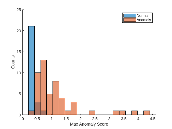
Plot a histogram of the maximum anomaly scores for the normal and anomalous classes. The distributions are well-separated by the model-predicted anomaly score.

numBins = 20;
[~,edges] = histcounts(scoresCal,numBins);
figure
hold on
hNormal = histogram(scoresCal(labelsCal==0),edges);
hAnomaly = histogram(scoresCal(labelsCal==1),edges);
hold off
legend([hNormal,hAnomaly],"Normal","Anomaly")
xlabel("Max Anomaly Score")
ylabel("Counts")

Calculate the optimal anomaly threshold by using the anomalyThreshold function. Specify the first two input arguments as the ground truth labels, labels, and predicted anomaly scores scores for the calibration data set. Specify the third input argument as true because true positive anomaly images have a labels value of true. The anomalyThreshold function returns the optimal threshold value as a scalar and the receiver operating characteristic (ROC) curve for the detector as an rocmetrics (Deep Learning Toolbox) object.

[thresh,roc] = anomalyThreshold(labelsCal,scoresCal,true);

Set the Threshold property of the anomaly detector to the optimal threshold value.

detector.Threshold = thresh;

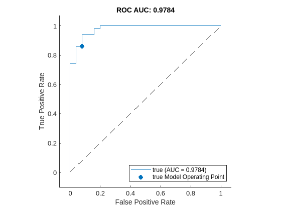
Plot the ROC curve by using the plot (Deep Learning Toolbox) object function of rocmetrics. The ROC curve illustrates the performance of the classifier for a range of possible threshold values. Each point on the ROC curve represents the false positive rate (x-coordinate) and true positive rate (y-coordinate) when you classify the calibration set images using a different threshold value. The solid blue line represents the ROC curve. The area under the ROC curve (AUC) metric indicates classifier performance, with a perfect classifier corresponding to the maximum ROC AUC 1.0.

plot(roc)
title("ROC AUC: " + roc.AUC)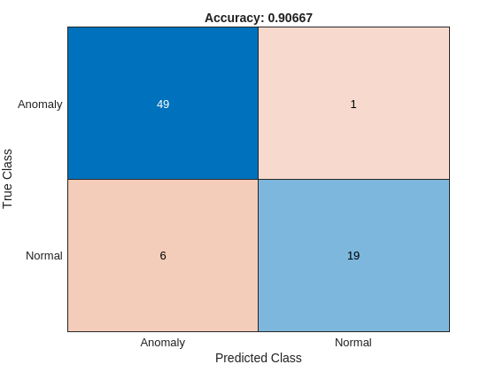

Evaluate Classification Model

Classify each image in the test set as either normal or anomalous by using the classify object function. Specify the MiniBatchSize argument as 1. Because the classify function evaluates the test images at full-size resolution, you must specify a small mini-batch size to prevent out-of-memory errors.

testSetPredictedLabels = classify(detector,dsTest,MiniBatchSize=1);
testSetPredictedLabels = testSetPredictedLabels';

Get the ground truth labels of each test image.

testSetGTLabels = dsTest.UnderlyingDatastores{1}.Labels ~= "good";

Evaluate the anomaly detector by calculating performance metrics using the evaluateAnomalyDetection function. The function calculates several metrics that evaluate the accuracy, precision, sensitivity, and specificity of the detector for the test data set.

metrics = evaluateAnomalyDetection(testSetPredictedLabels,testSetGTLabels,1);

Evaluating anomaly detection results
------------------------------------
* Finalizing... Done.
* Data set metrics:

    GlobalAccuracy    MeanAccuracy    Precision    Recall    Specificity    F1Score    FalsePositiveRate    FalseNegativeRate
    ______________    ____________    _________    ______    ___________    _______    _________________    _________________

       0.90667            0.87         0.89091      0.98        0.76        0.93333          0.24                 0.02       

The ConfusionMatrix property of metrics contains the confusion matrix for the test set. Extract the confusion matrix and display a confusion plot. The classification model in this example is very accurate and predicts a small percentage of false positives and false negatives.

M = metrics.ConfusionMatrix{:,:};
confusionchart(M,["Normal","Anomaly"])
acc = sum(diag(M))/sum(M,"all");
title("Accuracy: " + acc)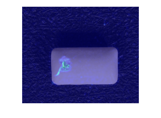

Explain Classification Decisions

You can use the anomaly score heatmap that the anomaly detector predicts to explain why the detector classifies an image as normal or anomalous. This approach is useful for identifying patterns in false negatives and false positives. You can use these patterns to identify strategies for increasing class balancing of the training data or improving the network performance.

Normalize Anomaly Heat Map Display Range

To compare anomaly scores observed across the entire calibration set, including normal and anomalous images, normalize the anomaly score map display range. By using the same display range across images, you can compare images more easily than if you scale each image to its own minimum and maximum.

Define a normalized display range, displayRange, that reflects the range of anomaly scores observed across the entire calibration set, including normal and anomalous images.

minMapVal = inf;
maxMapVal = -inf;
reset(dsCal)
while hasdata(dsCal)
    data = read(dsCal);
    img = data{1};
    map = anomalyMap(detector,img);
    minMapVal = min(min(map,[],"all"),minMapVal);
    maxMapVal = max(max(map,[],"all"),maxMapVal);
end
displayRange = [minMapVal 0.7*maxMapVal];

View Heatmap of Anomalous Image

Select an image of a correctly classified anomaly. Display the image, with the heatmap overlaid by using the anomalyMapOverlay function.

testSetAnomalyLabels = testSetGTLabels;
testSetOutputLabels = testSetPredictedLabels;
idxTruePositive = find(testSetAnomalyLabels & testSetOutputLabels);
dsExample = subset(dsTest,idxTruePositive);
data = read(dsExample);
img = data{1};
map = anomalyMap(detector,img);
imshow(anomalyMapOverlay(img,map,MapRange=displayRange,Blend="equal"))

View Heatmap of Normal Image

Select and display an image of a correctly classified normal image, with the heatmap overlaid by using the anomalyMapOverlay function.

idxTrueNegative = find(~(testSetAnomalyLabels | testSetOutputLabels));
dsExample = subset(dsTest,idxTrueNegative);
data = read(dsExample);
img = data{1};
map = anomalyMap(detector,img);
imshow(anomalyMapOverlay(img,map,MapRange=displayRange,Blend="equal"))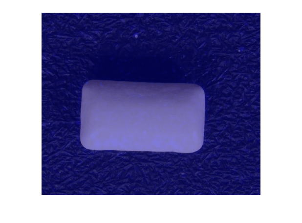

View Heatmap of False Positive Image

False positives are images without defects, but that the network misclassifies as anomalous. Use the explanation from the EfficientAD model [1] to gain insight into the misclassifications.

Select a false positive image, and display it, with the heatmap overlaid by using the anomalyMapOverlay function. For this test image, anomalous scores are localized to image areas with uneaven lightning, so you might consider adjusting the image contrast during preprocessing, increasing the number of images used for training, or choosing a different threshold at the calibration step.

idxFalsePositive = find(~(testSetAnomalyLabels) & testSetOutputLabels);
if ~isempty(idxFalsePositive)
    dsExample = subset(dsTest,idxFalsePositive);
    data = read(dsExample);
    img = data{1};
    map = anomalyMap(detector,img);
    figure
    imshow(anomalyMapOverlay(img,map,MapRange=displayRange,Blend="equal"))
end

View Heatmap of False Negative Image

False negatives are images with defects, but that the network misclassifies as normal. Use the explanation from the EfficientAD model [1] to gain insights into the misclassifications.

Select a false negative image, and display it, with the heatmap overlaid by using the anomalyMapOverlay function. To decrease false negative results, consider adjusting the anomaly threshold or CompressionRatio of the detector.

idxFalseNegative = find(testSetAnomalyLabels & (~testSetOutputLabels));
if ~isempty(idxFalseNegative)
    dsExample = subset(dsTest,idxFalseNegative);
    data = read(dsExample);
    img = data{1};
    map = anomalyMap(detector,img);
    figure
    imshow(anomalyMapOverlay(img,map,MapRange=displayRange,Blend="equal"))
end

Supporting Functions

addLabelData

The addLabelData helper function creates a one-hot encoded representation of label information in data.

function [data,info] = addLabelData(data,info)
    classNames = [info.Label];
    onehotencoding = classNames ~= categorical("good");
    data = {data,onehotencoding};
end

maskObjectsInNormalImages

The maskObjectsInNormalImages helper function creates a logical mask from a blocked image, in which true (or 1) pixels represent ROIs with meaningful normal data.

function bout = maskObjectsInNormalImages(bim,T)
    im = im2gray(bim.Data);

    % Threshold image using global threshold
    BW = imbinarize(im,T);

    % Morphologically open mask with square-shaped
    % structuring element
    width = 3;
    se = strel("square",width);
    BW = imopen(BW,se);

    bout = BW;
end

References

[1] Batzner, Kilian, Lars Heckler, and Rebecca König. “EfficientAD: Accurate Visual Anomaly Detection at Millisecond-Level Latencies.” In 2024 IEEE/CVF Winter Conference on Applications of Computer Vision (WACV), 127–37. Waikoloa, HI, USA: IEEE, 2024. https://doi.org/10.1109/WACV57701.2024.00020.

[2] Zou, Yang, Jongheon Jeong, Latha Pemula, Dongqing Zhang, and Onkar Dabeer. “SPot-the-Difference Self-Supervised Pre-Training for Anomaly Detection and Segmentation.” arXiv, July 28, 2022. https://doi.org/10.48550/arXiv.2207.14315.