Create Plot
Interactively visualize filter responses and other outputs for several signal processing functions
Since R2023a
Description
The Create Plot task lets you interactively visualize filter responses and other outputs for several signal processing functions in your MATLAB® workspace.
You can create a Create Plot task to visualize the outputs of these signal processing functions:
cwt(since R2026a)freqz(Signal Processing Toolbox)grpdelay(Signal Processing Toolbox)impz(Signal Processing Toolbox)periodogram(Signal Processing Toolbox)pspectrum(Signal Processing Toolbox)pwelch(Signal Processing Toolbox)spectrogram(Signal Processing Toolbox)zplane(Signal Processing Toolbox)
The functions covered in this task are available when you select
Signal Processing in the Filter by Category
menu in the Create Plot
Live Editor task. To learn more about Live Editor tasks, see Add Interactive Tasks to a Live Script.
Open the Task
To add the Create Plot task to a live script in the MATLAB Editor:
On the Live Editor tab, click Task > Create Plot.
In a code block in the live script, type a relevant keyword, such as
cwt,grpdelay,pspectrum, orspectrogram. Select Create Plot from the suggested command completions. When you add the task using this method, then MATLAB automatically selects the corresponding chart type in the Select visualization section of the task.
Examples
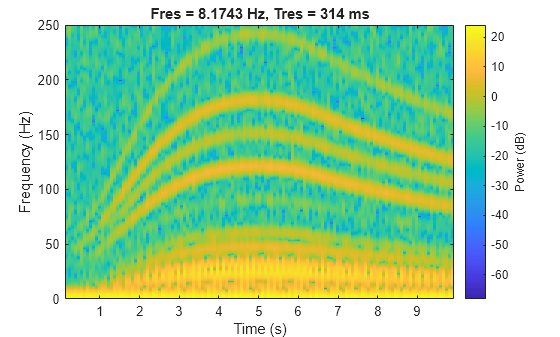
Use the Create Plot task in the Live Editor to interactively create and visualize the spectrogram of a vibrational signal.
Load the signal, vib, which measures vibration in a helicopter. The signal lasts for 10 seconds at a sample rate Fs of 500 Hz.
load helidataTo visualize the spectrogram using the pspectrum visualization:
Open the Create Plot task.
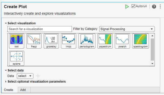
In the Filter by Category menu of the Select visualization section, select
Signal Processing. The gallery that appears shows several visualization functions that you can use to plot outputs related to signal processing.In the gallery, click the
pspectrumvisualization.Set the parameters for the visualization. Expand the Select data section.
Set Configuration to
Specify sample rate for spectrogram.Set Input signal to
vib.Set Sample rate to
fs.
To see the code that this task generates, expand the task display by clicking Show code at the bottom of the task parameter area.
% Create spectrogram estimate plot of vib


pspectrum(vib,fs,"spectrogram");
Use the Create Plot task in the Live Editor to interactively create and visualize the scalogram using the continuous wavelet transform.
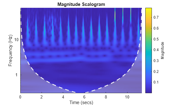
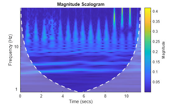
Load the electrocardiogram (ECG) signal into your workspace. The sample rate is 180 Hz.
load wecg
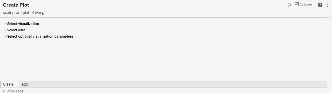
Fs = 180;To visualize the scalogram, open the Create Plot task. Start by typing the keyword cwt in a code block and then click Create Plot. Select the input signal and sample rate to plot the scalogram. By default, the cwt function uses the (3,60) analytic Morse wavelet
To see the code that this task generates, expand the task display by clicking ![]() Show code at the bottom of the task parameter area.
Show code at the bottom of the task parameter area.
Change Default Wavelet
To visualize the scalogram using the bump wavelet, open the Create Plot task. Start by typing the keyword cwt in a code block and then click Create Plot. Select the input signal and sample rate to plot the scalogram. Expand Select optional visualization parameters and select the bump wavelet.
To see the code that this task generates, expand the task display by clicking ![]() Show code at the bottom of the task parameter area.
Show code at the bottom of the task parameter area.

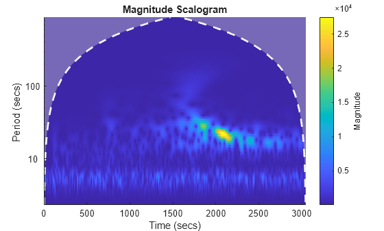
Specify Sample Time
Load the Kobe earthquake data. The sample time is 1 second.
load kobe
Ts = seconds(1);
To visualize the scalogram using the sample time, open the Create Plot task. Start by typing the keyword cwt in a code block and then click Create Plot. Select the configuration Specify signal with sample time for scalogram. Select the input signal and sample time to plot the scalogram.
To see the code that this task generates, expand the task display by clicking ![]() Show code at the bottom of the task parameter area.
Show code at the bottom of the task parameter area.

Parameters
Version History
Introduced in R2023aSee Also
Functions
cwt|freqz(Signal Processing Toolbox) |grpdelay(Signal Processing Toolbox) |impz(Signal Processing Toolbox) |periodogram(Signal Processing Toolbox) |pspectrum(Signal Processing Toolbox) |pwelch(Signal Processing Toolbox) |spectrogram(Signal Processing Toolbox) |zplane(Signal Processing Toolbox)