rlocus

Root locus of dynamic system

Syntax

[r,kout] = rlocus(sys)

r = rlocus(sys,k)

rlocus(___)

Description

[r,kout] = rlocus(sys) calculates the root locus of SISO model sys and returns the resulting vector of feedback gains k and corresponding complex root locations r.

To produce a smooth root locus, rlocus automatically selects a set of positive feedback gains.

For more information about the root locus of a dynamic system, see Algorithms.

example

r = rlocus(sys,k) returns the closed-loop poles corresponding to the feedback gains specified in k.

example

rlocus(___) plots the root locus of the SISO model sys with default plotting options for all of the previous input argument combinations. For more plot customization options, use rlocusplot.

To plot the root locus for multiple dynamic systems on the same plot, you can specify sys as a comma-separated list of models. For example, rlocus(sys1,sys2,sys3) plots the root locus for three models on the same plot.
To specify a color, line style, and marker for each system in the plot, specify a LineSpec value for each system. For example, rlocus(sys1,LineSpec1,sys2,LineSpec2) plots two models and specifies their plot style. For more information on specifying a LineSpec value, see rlocusplot.

Examples

collapse all

Root Locus Plot of Dynamic System

Open Live Script

For this example, plot the root-locus of the following SISO dynamic system:

$s y s (s) = \frac{2 s^{2} + 5 s + 1}{s^{2} + 2 s + 3} .$

sys = tf([2 5 1],[1 2 3]);
rlocus(sys)

MATLAB figure

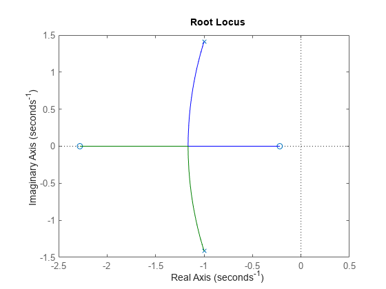
The poles of the system are denoted by x, while the zeros are denoted by o on the root locus plot. You can use the menu within the generated root locus plot to add grid lines, zoom in or out, and also invoke the Property Editor to customize the plot.

For more plot customization options, use rlocusplot.

Root Locus Plot of Multiple Dynamic System Models

Open Live Script

For this example, consider sisoModels.mat which contains the following three SISO models:

sys1 $-$ a transfer function model
sys2 $-$ a state-space model
sys3 $-$ a zero-pole-gain model

Load the models from the mat file.

load('sisoModels.mat','sys1','sys2','sys3');

Create the root locus plot using rlocus and specify the color for each system. Also add a legend to the root locus plot.

rlocus(sys1,'b',sys2,'k',sys3,'r')
hold on
legend('sys1','sys2','sys3')
hold off

MATLAB figure

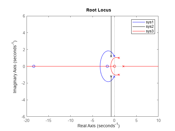
The figure contains root locus diagrams for all three systems in the same plot. For more plot customization, see rlocusplot.

Closed-Loop Poles and Feedback Gain Values Using Root Locus

Open Live Script

For this example, consider the following SISO transfer function model:

$s y s (s) = \frac{3 s^{2} + 1}{9 s^{3} + 7 s^{2} + 5 s + 6}$

Use the above transfer function model with rlocus to extract the closed-loop poles and associated feedback gain values.

sys = tf([3 0 1],[9 7 5 6]);
[r,k] = rlocus(sys)

r = 3×53 complex
10² ×

  -0.0094 + 0.0000i  -0.0104 + 0.0000i  -0.0105 + 0.0000i  -0.0106 + 0.0000i  -0.0107 + 0.0000i  -0.0108 + 0.0000i  -0.0109 + 0.0000i  -0.0111 + 0.0000i  -0.0112 + 0.0000i  -0.0113 + 0.0000i  -0.0115 + 0.0000i  -0.0117 + 0.0000i  -0.0119 + 0.0000i  -0.0121 + 0.0000i  -0.0124 + 0.0000i  -0.0126 + 0.0000i  -0.0129 + 0.0000i  -0.0132 + 0.0000i  -0.0135 + 0.0000i  -0.0139 + 0.0000i  -0.0143 + 0.0000i  -0.0148 + 0.0000i  -0.0152 + 0.0000i  -0.0158 + 0.0000i  -0.0163 + 0.0000i  -0.0170 + 0.0000i  -0.0177 + 0.0000i  -0.0184 + 0.0000i  -0.0192 + 0.0000i  -0.0201 + 0.0000i  -0.0211 + 0.0000i  -0.0222 + 0.0000i  -0.0233 + 0.0000i  -0.0246 + 0.0000i  -0.0259 + 0.0000i  -0.0274 + 0.0000i  -0.0290 + 0.0000i  -0.0307 + 0.0000i  -0.0326 + 0.0000i  -0.0346 + 0.0000i  -0.0368 + 0.0000i  -0.0392 + 0.0000i  -0.0418 + 0.0000i  -0.0446 + 0.0000i  -0.0476 + 0.0000i  -0.0508 + 0.0000i  -0.0543 + 0.0000i  -0.0582 + 0.0000i  -0.0623 + 0.0000i  -0.0667 + 0.0000i
   0.0008 + 0.0084i   0.0006 + 0.0083i   0.0006 + 0.0082i   0.0006 + 0.0082i   0.0006 + 0.0082i   0.0006 + 0.0082i   0.0005 + 0.0082i   0.0005 + 0.0082i   0.0005 + 0.0082i   0.0005 + 0.0081i   0.0005 + 0.0081i   0.0004 + 0.0081i   0.0004 + 0.0081i   0.0004 + 0.0080i   0.0004 + 0.0080i   0.0003 + 0.0080i   0.0003 + 0.0080i   0.0003 + 0.0079i   0.0002 + 0.0079i   0.0002 + 0.0078i   0.0002 + 0.0078i   0.0002 + 0.0078i   0.0001 + 0.0077i   0.0001 + 0.0077i   0.0001 + 0.0076i   0.0000 + 0.0076i   0.0000 + 0.0075i  -0.0000 + 0.0074i  -0.0000 + 0.0074i  -0.0000 + 0.0073i  -0.0001 + 0.0073i  -0.0001 + 0.0072i  -0.0001 + 0.0071i  -0.0001 + 0.0071i  -0.0001 + 0.0070i  -0.0001 + 0.0070i  -0.0001 + 0.0069i  -0.0001 + 0.0068i  -0.0001 + 0.0068i  -0.0001 + 0.0067i  -0.0001 + 0.0067i  -0.0001 + 0.0066i  -0.0001 + 0.0066i  -0.0001 + 0.0065i  -0.0001 + 0.0065i  -0.0001 + 0.0064i  -0.0001 + 0.0064i  -0.0001 + 0.0064i  -0.0001 + 0.0063i  -0.0001 + 0.0063i
   0.0008 - 0.0084i   0.0006 - 0.0083i   0.0006 - 0.0082i   0.0006 - 0.0082i   0.0006 - 0.0082i   0.0006 - 0.0082i   0.0005 - 0.0082i   0.0005 - 0.0082i   0.0005 - 0.0082i   0.0005 - 0.0081i   0.0005 - 0.0081i   0.0004 - 0.0081i   0.0004 - 0.0081i   0.0004 - 0.0080i   0.0004 - 0.0080i   0.0003 - 0.0080i   0.0003 - 0.0080i   0.0003 - 0.0079i   0.0002 - 0.0079i   0.0002 - 0.0078i   0.0002 - 0.0078i   0.0002 - 0.0078i   0.0001 - 0.0077i   0.0001 - 0.0077i   0.0001 - 0.0076i   0.0000 - 0.0076i   0.0000 - 0.0075i  -0.0000 - 0.0074i  -0.0000 - 0.0074i  -0.0000 - 0.0073i  -0.0001 - 0.0073i  -0.0001 - 0.0072i  -0.0001 - 0.0071i  -0.0001 - 0.0071i  -0.0001 - 0.0070i  -0.0001 - 0.0070i  -0.0001 - 0.0069i  -0.0001 - 0.0068i  -0.0001 - 0.0068i  -0.0001 - 0.0067i  -0.0001 - 0.0067i  -0.0001 - 0.0066i  -0.0001 - 0.0066i  -0.0001 - 0.0065i  -0.0001 - 0.0065i  -0.0001 - 0.0064i  -0.0001 - 0.0064i  -0.0001 - 0.0064i  -0.0001 - 0.0063i  -0.0001 - 0.0063i

k = 1×53

         0    0.4201    0.4542    0.4911    0.5309    0.5740    0.6205    0.6709    0.7253    0.7841    0.8477    0.9165    0.9908    1.0712    1.1581    1.2521    1.3536    1.4634    1.5822    1.7105    1.8493    1.9993    2.1614    2.3368    2.5263    2.7313    2.9529    3.1924    3.4514    3.7313    4.0340    4.3613    4.7151    5.0975    5.5111    5.9581    6.4415    6.9640    7.5289    8.1397    8.8000    9.5138   10.2856   11.1200   12.0220   12.9973   14.0516   15.1915   16.4238   17.7561

Since sys contains 3 poles, the size of the resultant array of poles r is 3x53. Each column in r corresponds to a gain value from vector k. For this example, rlocus automatically chose 53 values of k from zero to infinity to obtain a smooth trajectory for the three closed-loop poles.

display(r(:,39))

  -3.2585 + 0.0000i
  -0.0145 + 0.6791i
  -0.0145 - 0.6791i

display(k(39))

    7.5289

For instance, r(:,39) contains the above closed-loop poles for a feedback gain value of 7.5289.

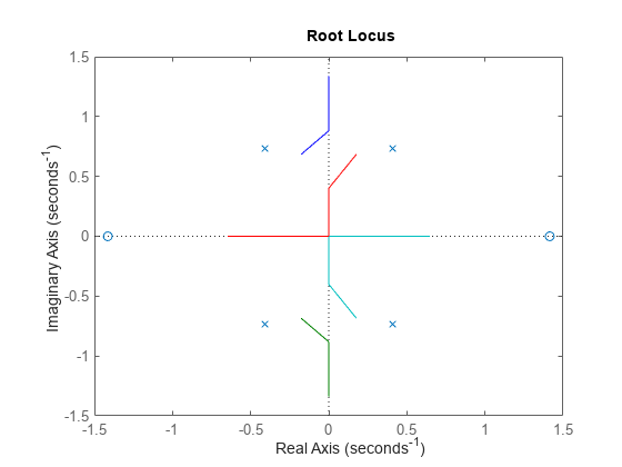
Closed-Loop Pole Locations for a Set of Feedback Gain Values

Open Live Script

For this example, consider the following SISO transfer function model:

$s y s (s) = \frac{0.5 s^{2} - 1}{4 s^{4} + 3 s^{2} + 2}$

Define the transfer function model and required vector of feedback gain values. For this example, consider a set of gain values varying from 1 to 8 with increments of 0.5 and extract the closed-loop pole locations using rlocus.

sys = tf([0.5 0 -1],[4 0 3 0 2]);
k = (1:0.5:5);
r = rlocus(sys,k);
size(r)

ans = 1×2

     4     9

Since sys contains 4 closed-loop poles, the size of the resultant array of closed-pole locations r is 4x9 where the 9 columns correspond to the 9 specific gain values defined in k.

You can also visualize the trajectory of the closed-loop poles for the specific gain values in k on the root locus plot.

rlocus(sys,k)

MATLAB figure

Input Arguments

collapse all

`sys` — Dynamic system
dynamic system model | model array

Dynamic system, specified as a SISO dynamic system model or array of dynamic system models. Dynamic systems that you can use include:

Continuous-time or discrete-time numeric LTI models, such as tf, zpk, or ss models.
Generalized or uncertain LTI models such as genss or uss (Robust Control Toolbox) models. Using uncertain models requires Robust Control Toolbox™ software.
- For tunable control design blocks, the function evaluates the model at its current value to plot the response.
- For uncertain control design blocks, the function plots the nominal value and random samples of the model.
Identified LTI models, such as idtf (System Identification Toolbox), idss (System Identification Toolbox), or idproc (System Identification Toolbox) models. Using identified models requires System Identification Toolbox™ software.

If sys is an array of models, the plot shows responses of all models in the array on the same axes.

`k` — Feedback gain values
vector

Feedback gain values that pertain to pole locations, specified as a vector. The feedback gains define the trajectory of the poles thereby affecting the shape of the root locus plot.

Output Arguments

collapse all

`r` — Closed-loop pole locations
array

Closed-loop pole locations of sys corresponding to each feedback gain value kout, returned as an N-by-M array, where N is the number of closed-loop poles of sys and M is the max(length(k)).

`kout` — Feedback gain values
vector

Feedback gain values that pertain to pole locations, returned as a vector. The feedback gains define the trajectory of the poles thereby affecting the shape of the root locus plot. When k is not defined by the user, rlocus adaptively selects a set of positive gains k between zero and infinity, to produce a smooth plot.

Tips

For an interactive approach to root locus plotting, see Control System Designer.
For additional options for customizing the appearance of the root locus plot, use rlocusplot.
Plots created using rlocus do not support multiline titles or labels specified as string arrays or cell arrays of character vectors. To specify multiline titles and labels, use a single string with a newline character.
```
rlocus(sys)
title("first line" + newline + "second line");
```

Algorithms

The root locus of a dynamic system contains the closed-loop pole trajectories as a function of the feedback gain k (assuming negative feedback). Root loci are used to study the effects of varying feedback gains on closed-loop pole locations. In turn, these locations provide indirect information on the time and frequency responses.

You can use rlocus to compute the root locus diagram of any of the following negative feedback loops by setting sys as shown below in the following figure.

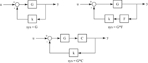
For instance, if sys is a transfer function represented by

$s y s (s) = \frac{n (s)}{d (s)}$

the closed-loop poles are the roots of

$d (s) + k n (s) = 0$

A root locus plot depicts the trajectories of the closed-loop poles as the feedback gain k varies from 0 to infinity.

Version History

Introduced before R2006a

expand all

R2024b: `gca` now returns chart object

For plots created using rlocus, the gca function now returns an rlocusplot chart object rather than an axes within the plot.

rlocus

Syntax

Description

Examples

Root Locus Plot of Dynamic System

Root Locus Plot of Multiple Dynamic System Models

Closed-Loop Poles and Feedback Gain Values Using Root Locus

Closed-Loop Pole Locations for a Set of Feedback Gain Values

Input Arguments

`sys` — Dynamic system
dynamic system model | model array

`k` — Feedback gain values
vector

Output Arguments

`r` — Closed-loop pole locations
array

`kout` — Feedback gain values
vector

Tips

Algorithms

Version History

R2024b: `gca` now returns chart object

See Also

Topics

rlocus

Syntax

Description

Examples

Root Locus Plot of Dynamic System

Root Locus Plot of Multiple Dynamic System Models

Closed-Loop Poles and Feedback Gain Values Using Root Locus

Closed-Loop Pole Locations for a Set of Feedback Gain Values

Input Arguments

sys — Dynamic system dynamic system model | model array

k — Feedback gain values vector

Output Arguments

r — Closed-loop pole locations array

kout — Feedback gain values vector

Tips

Algorithms

Version History

R2024b: gca now returns chart object

See Also

Topics

`sys` — Dynamic system
dynamic system model | model array

`k` — Feedback gain values
vector

`r` — Closed-loop pole locations
array

`kout` — Feedback gain values
vector

R2024b: `gca` now returns chart object