Quantization-Aware Training with Pseudo-Quantization Noise

Since R2026a

This example uses:

This example shows how to perform quantization-aware training (QAT) using the pseudo-quantization noise (PQN) injection technique with your deep neural network [1].

Injecting PQN into your network during training makes the network more robust against error introduced during quantization that reduces the accuracy of the quantized network. Quantization error is introduced when mapping a continuous range of values to a finite set of discrete steps. You can model quantization error using uniformly distributed data uncorrelated with the input signal [2]. This artificial quantization error is the PQN.

The PQN method involves retraining a fully trained network with a custom training loop that performs these actions:

Add artificial quantization error to the weights of the original network to create a temporary forward network.
Make predictions, calculate loss, and compute gradients using the forward network.
Update the weights of the original network using the gradient calculation from the forward network.

In this example, you start by transfer learning the MobileNet-V2 network to identify flowers from the flower data set [3], you retrain the network with QAT using the PQN method, and you then quantize the network.

QAT can take a considerable amount of time, so a GPU is recommended for this example. For more information about prerequisites for quantization of deep neural networks with a GPU, see Quantization Workflow System Requirements.

Load Flower Data Set

Download the flower data set using the downloadFlowerDataset supporting function included at the end of this example.

imageFolder = downloadFlowerDataset;
imds = imageDatastore(imageFolder, ...
        IncludeSubfolders=true, ...
        LabelSource="foldernames");

Inspect the classes of the data.

classes = string(categories(imds.Labels))

classes = 5×1 string array
    "daisy"
    "dandelion"
    "roses"
    "sunflowers"
    "tulips"

Perform Transfer Learning on MobileNet-V2

MobileNet-V2 is a convolutional neural network 53 layers deep. The pretrained version of the network is trained on more than a million images from the ImageNet database. For more information about MobileNet-V2, see Pretrained Deep Neural Networks.

Load the network.

net = imagePretrainedNetwork("mobilenetv2");

Split the data into training and validation sets. Create augmented image datastores that automatically resize the images to the input size of the network.

[imdsTrain,imdsValidation] = splitEachLabel(imds,0.9);
inputSize = net.Layers(1).InputSize;
augimdsTrain = augmentedImageDatastore(inputSize,imdsTrain);
augimdsValidation = augmentedImageDatastore(inputSize,imdsValidation);

Set aside a portion of the training data set to use during the calibration step of quantization. This data store should be representative of the data used for training and separate from the data set used to validate.

augimdsCalibration = subset(shuffle(augimdsTrain),1:320);

Perform transfer learning on the network using the flowers image data set with the createFlowerNetwork supporting function. The learnable parameters of the trained network transferNet are in single precision. For more information about transfer learning, see Retrain Neural Network to Classify New Images.

transferNet = createFlowerNetwork(net,augimdsTrain,augimdsValidation,classes);

Evaluate Baseline Network Performance

Evaluate the performance of the single-precision network using the testnet function. Performance in this case is defined as the correct classification rate.

accuracyOriginalNet = testnet(transferNet,augimdsValidation,"accuracy")

accuracyOriginalNet = 
91.0082

Quantize and evaluate the accuracy of the network before QAT to get a baseline performance for the fixed-point version of the network. The createQuantizedNetwork supporting function performs the same quantization workflow and is the function you use to quantize networks throughout the rest of the example.

Create a dlquantizer object and specify the network to quantize. Set the execution environment to GPU.

quantObj = dlquantizer(transferNet,ExecutionEnvironment="GPU");

Simulate and collect ranges of the network with a representative datastore using calibrate.

calibrate(quantObj,augimdsCalibration,UseGPU='auto');

Quantize the network using quantize.

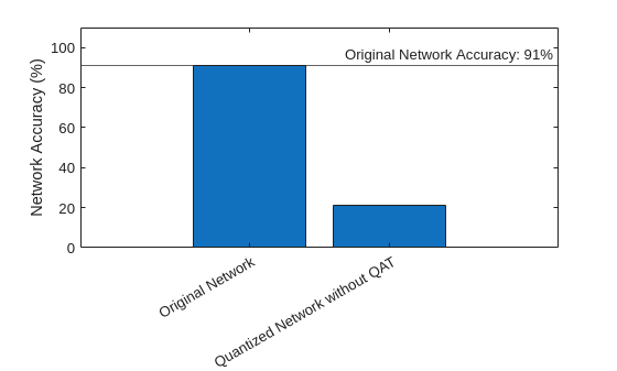
qOriginalNet = quantize(quantObj,ExponentScheme="Histogram");

Evaluate the performance of the fixed-point quantized network. There are five possible labels, so an accuracy value of 20% is equivalent to randomly guessing. Networks like MobileNet-V2 are sensitive to quantization due to the significant variation in range of values of the weight tensor of the convolution and grouped convolution layers.

accuracyOriginalQuantized = testnet(qOriginalNet,augimdsValidation,"accuracy")

accuracyOriginalQuantized = 
21.2534

Compare the accuracy of the floating- and fixed-point versions of the network before QAT.

figure
bar( ...
    ["Original Network","Quantized Network without QAT"], ...
    [accuracyOriginalNet,accuracyOriginalQuantized] ...
    )
xtickangle(30)
ylabel("Network Accuracy (%)")
ylim([0 110])
yline(accuracyOriginalNet,"-","Original Network Accuracy: "+round(accuracyOriginalNet)+"%")

Explore Effects of PQN on Network Layers

You can use an example output to explore how PQN can align with quantization error. The PQN is uniformly distributed noise uncorrelated with the input data, but this section shows it behaves similarly to the actual quantization error.

This example uses a 2D convolution layer. Adjust the layerIndex value to explore the PQN for different layers in the network.

fusedNet = fuseConvolutionAndBatchNormalizationLayers(transferNet);

allWeightsLayerIdx = find(arrayfun(@(layer) isprop(layer,'Weights'),fusedNet.Layers));
layerIndex = allWeightsLayerIdx(4)

layerIndex = 
7

layerName = fusedNet.Layers(layerIndex)

layerName = 
  Convolution2DLayer with properties:

              Name: 'block_1_expand'

   Hyperparameters
        FilterSize: [1 1]
       NumChannels: 16
        NumFilters: 96
            Stride: [1 1]
    DilationFactor: [1 1]
       PaddingMode: 'same'
       PaddingSize: [0 0 0 0]
      PaddingValue: 0

   Learnable Parameters
           Weights: [1×1×16×96 single]
              Bias: [1×1×96 single]

  Show all properties

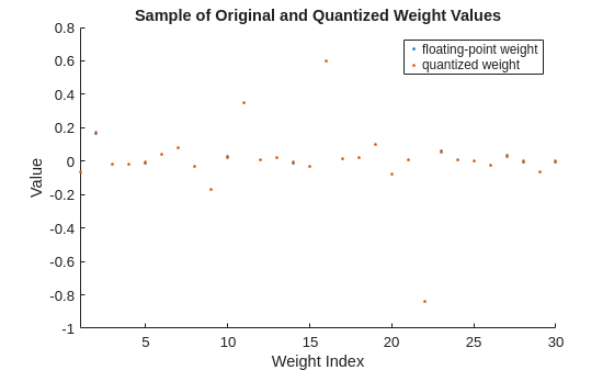
Display a sample of floating- and fixed-point weight values for the selected layer. The quantization error for each individual weight value is generally small and can err in either direction.

originalLayerWeights = fusedNet.Layers(layerIndex).Weights;
originalLayerWeights = reshape(originalLayerWeights,1,[]);
quantizedLayerWeights = fi(originalLayerWeights,1,8);

figure
sampleOriginalLayerWeights = randsample(originalLayerWeights,min(30,numel(originalLayerWeights)));
sampleQuantizedLayerWeights = fi(sampleOriginalLayerWeights,1,8);
scatter(1:numel(sampleOriginalLayerWeights),sampleOriginalLayerWeights,'.')
hold on
scatter(1:numel(sampleQuantizedLayerWeights),sampleQuantizedLayerWeights,'.')
xlim("tight")
ylabel("Value")
xlabel("Weight Index")
title("Sample of Original and Quantized Weight Values")
legend("floating-point weight","quantized weight")
hold off

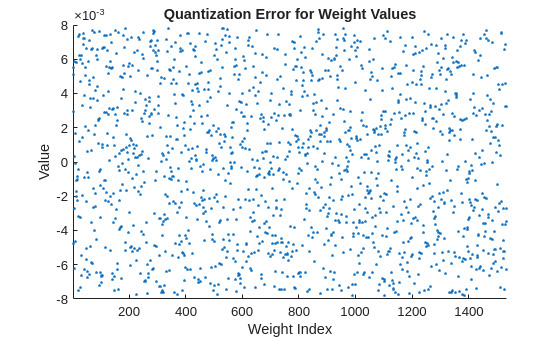
Display the quantization error between floating- and fixed-point weights values for all weights in the selected layer. Visually, the quantization error appears to be fairly uniform and random in its distribution.

figure
diffFQ = originalLayerWeights - cast(quantizedLayerWeights,"like",originalLayerWeights);
scatter(1:numel(originalLayerWeights),diffFQ,'.')
xlim("tight")
ylabel("Value")
xlabel("Weight Index")
title("Quantization Error for Weight Values")

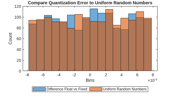
Compare the quantization error to random noise with values in the same range as the quantization error.

pqn = calculatePQN(originalLayerWeights);
limits= [min([diffFQ pqn],[],"all") max([diffFQ pqn],[],"all")];
numBins = 16;
figure
histogram(diffFQ,numBins,BinLimits=limits)
hold on
histogram(pqn,numBins,BinLimits=limits)
ylabel("Count")
xlabel("Bins")
title("Compare Quantization Error to Uniform Random Numbers")
legend("Difference Float vs Fixed","Uniform Random Numbers",Orientation="horizontal",Location="southoutside")
hold off;

Perform QAT with PQN

Quantization-aware training with PQN follows a similar structure as a standard custom training loop.

Initialize network parameters $θ$ to the fully trained floating-point network.
Define hyperparameters for training, such as learning rate and number of epochs.
Before each iteration, adjust weights for each layer by adding PQN creating the modified parameters $θ^{'} .$
Compute predictions using modified parameters $θ^{'}$ and loss between predictions and ground truth.
Update the original parameters $θ$ using gradients calculated for the loss with respect to the adjusted parameters $θ^{'} .$

Specify training options. These options have been determined through experimentation for this particular network.

QATnet = fusedNet;
numEpochs = 30;
miniBatchSize = 64;
learnRate = 2.15e-3;
momentum = 0.25;

accfun = dlaccelerate(@modelLoss);
clearCache(accfun);

Generate a minibatchqueue object to prepare the data for training. The minibatchqueue object prepares mini-batches of images and classification labels that help manage data in a custom training loop.

mbq = minibatchqueue(augimdsTrain,...
    MiniBatchSize=miniBatchSize,...
    MiniBatchFcn=@preprocessMiniBatch,...
    OutputEnvironment="auto", ...
    MiniBatchFormat=["SSCB" ""], ...
    PartialMiniBatch="discard");

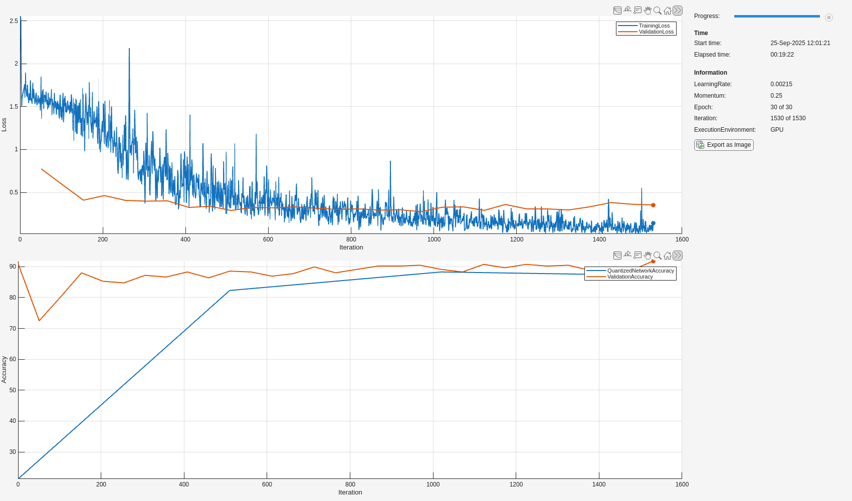
Set up the training progress monitor. This process creates one plot with the training loss and validation loss and one plot with the accuracy of the quantized network and the accuracy of the single-precision floating-point network.

monitor = trainingProgressMonitor( ...
    Metrics=["TrainingLoss","ValidationLoss","ValidationAccuracy","QuantizedNetworkAccuracy"], ...
    Info = ["LearningRate","Momentum","Epoch","Iteration","ExecutionEnvironment"],  ...
    XLabel="Iteration");

groupSubPlot(monitor, Loss=["TrainingLoss","ValidationLoss"]);
groupSubPlot(monitor, Accuracy=["QuantizedNetworkAccuracy","ValidationAccuracy"]);

Set the execution environment and record this information in the training progress monitor using the updateInfo function.

executionEnvironment = "auto";

if (executionEnvironment == "auto" && canUseGPU) || executionEnvironment == "gpu"
    updateInfo(monitor,ExecutionEnvironment="GPU");
else
    updateInfo(monitor,ExecutionEnvironment="CPU");
end

Record metrics for the training network and the quantized network before training.

originalValidationAccuracy = testnet(QATnet,augimdsValidation,"accuracy");
recordMetrics(monitor,0,ValidationAccuracy=originalValidationAccuracy);
recordMetrics(monitor,0,QuantizedNetworkAccuracy=accuracyOriginalQuantized);

Keep track of the network with the highest accuracy during the QAT.

bestQATnet = QATnet;
bestQuantizedNetworkAccuracy = accuracyOriginalQuantized;

Train the network.

numObservationsTrain = numel(augimdsTrain.Files);
numIterationsPerEpoch = floor(numObservationsTrain / miniBatchSize);
numIterations = numEpochs * numIterationsPerEpoch;

epoch = 0;
iteration = 0;
velocity = []; % for sgdm

while epoch < numEpochs && ~monitor.Stop
    
    epoch = epoch + 1;
    shuffle(mbq);

    while hasdata(mbq) && ~monitor.Stop
        iteration = iteration + 1;

        % Capture original network parameters
        originalParam = QATnet.Learnables;
        
        % Add Pseudo Quantization Noise to original network
        QATNetWithPQN = addNoiseToLearnables(QATnet); 

        [X,T] = next(mbq);       

        [loss,gradients,state] = dlfeval(accfun,QATNetWithPQN,X,T);
        QATnet.State = state;

        % Update original network parameters using SGDM using gradients
        % derived from the network with quantization error added
        [updatedParam,velocity] = sgdmupdate(originalParam,gradients,velocity,learnRate,momentum); 
        QATnet.Learnables = updatedParam; 

        % Record training loss
        recordMetrics(monitor,iteration,TrainingLoss=loss);
        updateInfo(monitor, ...
            LearningRate=learnRate, ...
            Momentum = momentum, ...
            Epoch=string(epoch) + " of " + string(numEpochs), ...
            Iteration=string(iteration) + " of " + string(numIterations));
        monitor.Progress = 100 * iteration/numIterations;
        
    end

    % Record validation loss
    epochValidationLoss = testnet(QATnet,augimdsValidation,"crossentropy");
    recordMetrics(monitor,iteration,ValidationLoss=epochValidationLoss);
   
    % Record validation accuracy of QAT network
    epochValidationAccuracy = testnet(QATnet,augimdsValidation,"accuracy");
    recordMetrics(monitor,iteration,ValidationAccuracy=epochValidationAccuracy);

    % Check every 10 epochs to validate performance of quantized network
    if mod(epoch, 10) == 0 || epoch == numEpochs
        qQATnet = createQuantizedNetwork(QATnet,augimdsCalibration);
        quantizedNetworkEpochAccuracy = testnet(qQATnet,augimdsValidation,"accuracy");
        recordMetrics(monitor,iteration,QuantizedNetworkAccuracy=quantizedNetworkEpochAccuracy);

        % Update bestQATnet with best performing quantized network
        if quantizedNetworkEpochAccuracy > bestQuantizedNetworkAccuracy
            bestQuantizedNetworkAccuracy = quantizedNetworkEpochAccuracy;
            bestQATnet = QATnet;
        end
    end
    

end

Evaluate Quantized Network

Evaluate the performance of the quantized network with QAT.

quantizedQATNet = createQuantizedNetwork(bestQATnet,augimdsCalibration);
accuracyQATQuantized = testnet(quantizedQATNet,augimdsValidation,"accuracy")

accuracyQATQuantized = 
88.2834

Compare the accuracy of the quantized networks with and without QAT.

figure
bar( ...
    ["Original Network","Quantized Network without QAT","Quantized Network with QAT"], ...
    [accuracyOriginalNet,accuracyOriginalQuantized,accuracyQATQuantized] ...
    )
ylabel("Network Accuracy (%)")
ylim([0 110])
yline(accuracyOriginalNet,"-","Original Network Accuracy: " + round(accuracyOriginalNet) + "%")

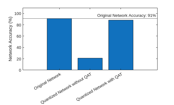
With QAT, the quantized network has a very small decrease in accuracy compared to the floating-point network.

Supporting Functions

Download Flower Data Set

The downloadFlowerDataset function downloads and extracts the flowers data set, if the data set is not yet in the current folder.

function imageFolder = downloadFlowerDataset

    downloadFolder = pwd;
    filename = fullfile(downloadFolder,"flower_dataset.tgz");
    imageFolder = fullfile(downloadFolder,"flower_photos");

    if ~exist(imageFolder,"dir")
        disp("Downloading Flower Dataset (218 MB)...")
        url = "http://download.tensorflow.org/example_images/flower_photos.tgz";
        websave(filename,url);
        untar(filename,downloadFolder)
    end

end

Perform Transfer Learning

The createFlowerNetwork function replaces the final fully connected and classification layer of the MobileNet-V2 network and retrains the network to classify flowers. For more information about MobileNet-V2, see Pretrained Deep Neural Networks.

function transfer_net = createFlowerNetwork(net,augimdsTrain,augimdsValidation,classes)

    downloadFolder = pwd;
    transferNetPath = fullfile(downloadFolder,"transfer_net.mat");

    if ~exist(transferNetPath,"file")
        % Define a new learnable fully connected layer
        learnRateFactor = 10;
        numClasses = numel(classes);
        newLearnableLayer = fullyConnectedLayer(numClasses, ...
            Name="new_fc", ...
            WeightLearnRateFactor=learnRateFactor, ...
            BiasLearnRateFactor=learnRateFactor);

        % Replace the last learnable layer with a new one.
        net = replaceLayer(net,"Logits",newLearnableLayer);

        % Specify training options.
        miniBatchSize = 64;
        validationFrequencyEpochs = 1;
        numObservations = augimdsTrain.NumObservations;
        numIterationsPerEpoch = floor(numObservations/miniBatchSize);
        validationFrequency = validationFrequencyEpochs * numIterationsPerEpoch;

        options = trainingOptions("sgdm", ...
            MaxEpochs=5, ...
            MiniBatchSize=miniBatchSize, ...
            InitialLearnRate=3e-4, ...
            Shuffle="every-epoch", ...
            ValidationData=augimdsValidation, ...
            ValidationFrequency=validationFrequency, ...
            Metrics = "accuracy", ...
            Plots="none", ...
            Verbose=false);

        % Train the network.
        transfer_net = trainnet(augimdsTrain,net,"crossentropy",options);
        save(transferNetPath,'transfer_net');
    end

    load(transferNetPath,'transfer_net');
end

Fuse Convolution and Batch Normalization Layers

The fuseConvolutionAndBatchNormalizationLayers function fuses batch normalization layers of the network to the preceding convolution layer. To use this function, your network layers must be in topological order.

function fusedNet = fuseConvolutionAndBatchNormalizationLayers(originalNet)
    fusedNet = originalNet;

    for idx = 1:numel(originalNet.Layers) - 1
        currentLayer = originalNet.Layers(idx);
        nextLayer = originalNet.Layers(idx + 1);

        % Find 2-D convolution layers or 2-D grouped convolution layers.
        if (isa(currentLayer,"nnet.cnn.layer.Convolution2DLayer") ...
                || isa(currentLayer,"nnet.cnn.layer.GroupedConvolution2DLayer")) ...
            && isa(nextLayer,"nnet.cnn.layer.BatchNormalizationLayer")

            % Replace convolution layer with a convolution layer with learnables 
            % adjusted with BatchNormalization statistics.
            [adjustedWeights, adjustedBias] = foldBatchNormalizationParameters( ...
                currentLayer.Weights,currentLayer.Bias, ...
                nextLayer.Offset,nextLayer.Scale,nextLayer.TrainedMean,nextLayer.TrainedVariance,nextLayer.Epsilon);
            currentLayer.Weights = adjustedWeights;
            currentLayer.Bias = adjustedBias;

            currentLayerName = string(currentLayer.Name);
            nextLayerName = string(nextLayer.Name);
            fusedNet = groupLayers(fusedNet,[currentLayerName,nextLayerName],GroupNames=currentLayerName);
            fusedNet = replaceLayer(fusedNet,currentLayerName,currentLayer,ReconnectBy="order");
        end
    end
    fusedNet = initialize(fusedNet);
end

Create Quantized Network

Define the createQuantizedNetwork helper function. This function constructs a dlquantizer object for GPU target, simulates and collects ranges of the network with a representative datastore using the calibrate function, and then quantizes the network using the quantize function.

function qNet = createQuantizedNetwork(net,calDS,exponentScheme,executionEnvironment)
    arguments
        net 
        calDS 
        exponentScheme = "Histogram"
        executionEnvironment = "GPU"
    end
    dq = dlquantizer(net,ExecutionEnvironment=executionEnvironment);
    calibrate(dq,calDS,UseGPU='auto');
    qNet = quantize(dq,ExponentScheme=exponentScheme);
end

Calculate Loss and Gradients

The modelLoss function calculates the loss and gradients of the training to aid in acceleration of the training.

function [loss,gradients,state] = modelLoss(net,X,T)
        
    % Forward data through network.
    [Y, state] = forward(net,X);
    
    % Calculate cross-entropy loss.
    loss = crossentropy(Y,T);
    
    % Calculate gradients of loss with respect to learnable parameters.
    gradients = dlgradient(loss,net.Learnables);

end

Preprocess Mini-Batch

The preprocessMiniBatch function preprocesses the input data for the mini-batch queue.

function [X,T] = preprocessMiniBatch(dataX,dataT)
    X = cat(4, dataX{:}); 
    T = cat(2, dataT{:});   
    T = onehotencode(T, 1);
end

Add Pseudo-Quantization Noise to Network

For each layer in the network with a Weights parameter, the addNoiseToLearnables function adds noise to the learnable to mimic quantization error.

function net = addNoiseToLearnables(net)
    learnables = net.Learnables;
    learnableValues = learnables.Value;
    for idx = 1:height(learnableValues)
        if learnables.Parameter(idx) == "Weights"
            learnableValues{idx} = learnableValues{idx} + calculatePQN(learnableValues{idx});
        end
    end
    net.Learnables.Value = learnableValues;
end

Calculate Pseudo-Quantization Noise

The calculatePQN function generates a matrix of uniformly distributed random numbers in the interval (-0.5, 0.5) scaled by the slope of a signed 8-bit fixed-point type that avoids overflows and maximizes precision.

function pqn = calculatePQN(value)
    if isdlarray(value)
        value = extractdata(value);
    end

    pqn = (rand(size(value))-0.5) .* getBestPrecisionScalingFactor(value, 1, 8);
end

Calculate Best-Precision Scaling Factor

Use the getBestPrecisionScalingFactor function to calculate the best-precision scaling factor. Given a value, the scaling factor is equal to slope of a fixed-point value that captures the range of value and assigns the remaining bits to use for precision.

function scalingFactor = getBestPrecisionScalingFactor(value,signedness,wordlength)
    maxValue = gather(max(abs(value),[],"all")); 
    
    scalingExponent = floor(log2(maxValue))-(wordlength - signedness - 1);
    scalingFactor = 2^scalingExponent;
end

References

[1] Défossez, Alexandre, Yossi Adi, and Gabriel Synnaeve. "Differentiable model compression via pseudo quantization noise." Transactions on Machine Learning Research (Sept. 2022): 1-16.

[2] Widrow, Bernard, Istvan Kollar, and Ming-Chang Liu. "Statistical theory of quantization." IEEE Transactions on Instrumentation and Measurement 45, no.2 (1996): 353-61.

[3] The TensorFlow Team. "Flowers." January 2019. http://download.tensorflow.org/example_images/flower_photos.tgz.