Train Network with LSTM Projected Layer
Train a deep learning network with an LSTM projected layer for sequence-to-label classification.
To compress a deep learning network, you can use projected layers. The layer introduces learnable projector matrices , replaces multiplications of the form , where is a learnable matrix, with the multiplication , and stores and instead of storing . Projecting into a lower dimensional space using typically requires less memory to store the learnable parameters and can have similarly strong prediction accuracy.
Reducing the number of learnable parameters by projecting an LSTM layer rather than reducing the number of hidden units of the LSTM layer maintains the output size of the layer and, in turn, the sizes of the downstream layers, which can result in better prediction accuracy.
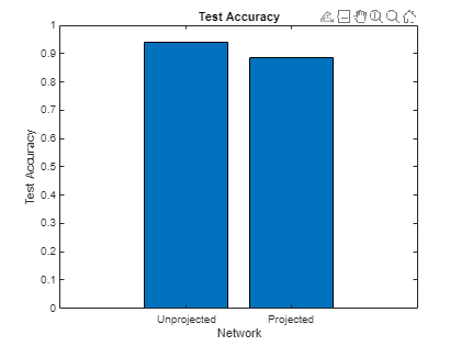
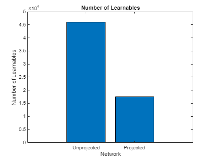
These charts compare the test accuracy and the number of learnable parameters of the LSTM network and the projected LSTM network that you train in this example.

In this example, you train an LSTM network for sequence classification, then train an equivalent network with an LSTM projected layer. You then compare the test accuracy and the number of learnable parameters for each of the networks.
Load Training Data
Load the Japanese Vowels data set described in [1] and [2] that contains 270 sequences of varying length with 12 features corresponding to LPC cepstrum coefficients and a categorical vector of labels 1, 2, ..., 9. The sequences are matrices with 12 rows (one row for each feature) and a varying number of columns (one column for each time step).
load japaneseVowelsTrainData.matVisualize the first time series in a plot. Each line corresponds to a feature.
figure
plot(XTrain{1}')
title("Training Observation 1")
numFeatures = size(XTrain{1},1);
legend("Feature " + string(1:numFeatures),Location="northeastoutside")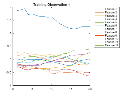
Define Network Architecture
Define the LSTM network architecture.
Specify a sequence input layer with an input size matching the number of features of the input data.
Specify an LSTM layer with 100 hidden units that outputs the last element of the sequence.
Specify a fully connected layer of a size equal to the number of classes, followed by a softmax layer.
inputSize = 12;
numHiddenUnits = 100;
numClasses = 9;

layers = [ ...
    sequenceInputLayer(inputSize)
    lstmLayer(numHiddenUnits,OutputMode="last")
    fullyConnectedLayer(numClasses)
    softmaxLayer];
Specify Training Options
Specify the training options.
Train using the Adam solver.
Train with a mini-batch size of 27 for 50 epochs.
Because the training data has sequences with rows and columns corresponding to channels and time steps, respectively, specify the input data format
"CTB"(channel, time, batch).Because the mini-batches are small with short sequences, the CPU is better suited for training. Train using the CPU.
Display the training progress in a plot and suppress the verbose output.
maxEpochs = 50;
miniBatchSize = 27;

options = trainingOptions("adam", ...
    MiniBatchSize=miniBatchSize, ...
    MaxEpochs=maxEpochs, ...
    InputDataFormats="CTB", ...
    ExecutionEnvironment="cpu", ...
    Plots="training-progress", ...
    Verbose=false);
Train Network
Train the neural network using the trainnet function. For classification, use cross-entropy loss. By default, the trainnet function uses a GPU if one is available. Training on a GPU requires a Parallel Computing Toolbox™ license and a supported GPU device. For information on supported devices, see GPU Computing Requirements (Parallel Computing Toolbox). Otherwise, the trainnet function uses the CPU. To specify the execution environment, use the ExecutionEnvironment training option.
net = trainnet(XTrain,TTrain,layers,"crossentropy",options);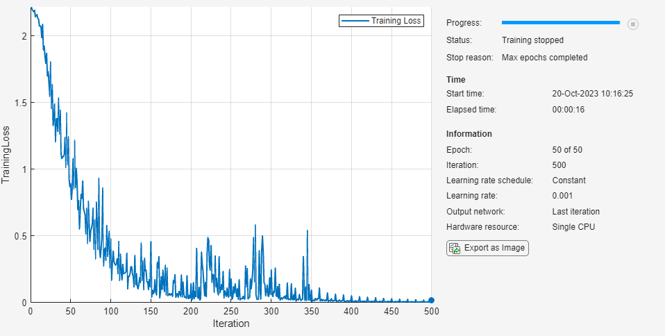
Test Network
Classify the test images. To make predictions with multiple observations, use the minibatchpredict function. To covert the prediction scores to labels, use the scores2label function. The minibatchpredict function automatically uses a GPU if one is available. Using a GPU requires a Parallel Computing Toolbox™ license and a supported GPU device. For information on supported devices, see GPU Computing Requirements (Parallel Computing Toolbox). Otherwise, the function uses the CPU.
Because the data has sequences with rows and columns corresponding to channels and time steps, respectively, specify the input data format "CTB" (channel, time, batch).
load japaneseVowelsTestData.mat
scores = minibatchpredict(net,XTest,MiniBatchSize=miniBatchSize,InputDataFormats="CTB");
YTest = scores2label(scores,categories(TTest));
acc = sum(YTest == TTest)./numel(TTest)
acc = 0.9405
View the number of learnables of the network using the analyzeNetwork function.
analyzeNetwork(net)
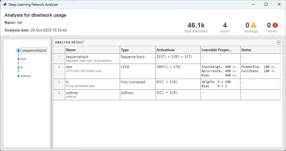
In order to compare the total number of learnable parameters of each network, store the total number of learnable parameters in a variable.
totalLearnables = 46100;
Train Projected LSTM Network
Create an identical network with an LSTM projected layer in place of the LSTM layer.
For the LSTM projected layer:
Specify the same number of hidden units as the LSTM layer
Specify an output projector size of 25% of the number of hidden units.
Specify an input projector size of 75% of the input size.
Ensure that the output and input projector sizes are positive by taking the maximum of the sizes and 1.
outputProjectorSize = max(1,floor(0.25*numHiddenUnits));
inputProjectorSize = max(1,floor(0.75*inputSize));

layersProjected = [ ...
    sequenceInputLayer(inputSize)
    lstmProjectedLayer(numHiddenUnits,outputProjectorSize,inputProjectorSize,OutputMode="last")
    fullyConnectedLayer(numClasses)
    softmaxLayer];
Train the projected LSTM network with the same data and training options.
netProjected = trainnet(XTrain,TTrain,layersProjected,"crossentropy",options);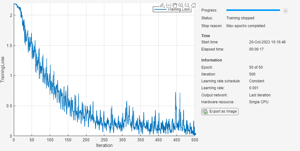
Test Projected Network
Calculate the classification accuracy of the predictions on the test data.
scores = minibatchpredict(netProjected,XTest,MiniBatchSize=miniBatchSize,InputDataFormats="CTB");
YTest = scores2label(scores,categories(TTest));
accProjected = sum(YTest == TTest)./numel(TTest)
accProjected = 0.8865
View the number of learnables of the network using the analyzeNetwork function.
analyzeNetwork(netProjected)

In order to compare the total number of learnable parameters of each network, store the total number of learnable parameters in a variable.
totalLearnablesProjected = 17500;
Compare Networks
Compare the test accuracy and number of learnables in each network. Depending on the projection sizes, the projected network can have significantly fewer learnable parameters and still maintain strong prediction accuracy.
Create a bar chart showing the test accuracy of each network.
figure
bar([acc accProjected])
xticklabels(["Unprojected","Projected"])
xlabel("Network")
ylabel("Test Accuracy")
title("Test Accuracy")
Create a bar chart showing the test accuracy the number of learnables of each network.
figure
bar([totalLearnables totalLearnablesProjected])
xticklabels(["Unprojected","Projected"])
xlabel("Network")
ylabel("Number of Learnables")
title("Number of Learnables")
Bibliography
M. Kudo, J. Toyama, and M. Shimbo. "Multidimensional Curve Classification Using Passing-Through Regions." Pattern Recognition Letters. Vol. 20, No. 11–13, pages 1103–1111.
UCI Machine Learning Repository: Japanese Vowels Dataset. https://archive.ics.uci.edu/ml/datasets/Japanese+Vowels
See Also
lstmProjectedLayer | trainnet | trainingOptions | dlnetwork | sequenceInputLayer | lstmLayer | bilstmLayer | gruLayer | convolution1dLayer
Topics
- Sequence Classification Using Deep Learning
- Sequence Classification Using 1-D Convolutions
- Compare Deep Learning and ARMA Models for Time Series Modeling
- Time Series Forecasting Using Deep Learning
- Sequence-to-One Regression Using Deep Learning
- Classify Videos Using Deep Learning
- Long Short-Term Memory Neural Networks
- List of Deep Learning Layers
- Deep Learning Tips and Tricks