simsmooth

R2026b

Simulation smoother for Bayesian linear state-space model

Since R2026b

collapse all in page

Syntax

X = simsmooth(PriorMdl,Y,params)

X = simsmooth(PriorMdl,Y,params,Name=Value)

[X,Parameters] = simsmooth(___)

Description

X = simsmooth(PriorMdl,Y,params) returns 1000 randomly drawn state paths, simulated from the posterior smoothed state distribution, by applying the standard simulation smoother (forward-filtering, backward-smoothing method) to the prior Bayesian linear state-space model PriorMdl and responses data Y. simsmooth computes the posterior distribution of the states conditioned on the state-space model parameters params. This computation does not incorporate parameter uncertainty.

When simsmooth simulates paths from the posterior smoothing distribution conditioned on model parameters, the state disturbances and observation innovations are Gaussian, regardless of the values of the StateDistribution and ObservationDistribution properties of PriorMdl. To simulate state paths from non-Gaussian models, set Joint=true.

example

X = simsmooth(PriorMdl,Y,params,Name=Value) specifies additional options using one or more name-value arguments. For example, simsmooth(PriorMdl,Y,params,NumDraws=1e4,Joint=true) specifies to generate 1e4 random draws from the posterior, and to sample from the joint posterior distribution of the smoothed states and state-space model parameters.

example

[X,Parameters] = simsmooth(___) additionally returns one of the following quantities in Parameters using any of the input argument combinations in the previous syntaxes:

When Joint=true, Parameters contains random draws of state-space model parameters from the joint posterior distribution of the states and model parameters. The function applies the forward-filtering, backward-sampling method.
When Joint=false (the default), Parameters contains the input params concatenated horizontally to produce a matrix with NumDraws repeated columns.

example

Examples

collapse all

Estimate Posterior Smoothing Conditional Distribution

Open Live Script

Estimate the posterior smoothing distribution of the states of a Bayesian state-space model, conditioned on the full data set and model parameters. This example simulates observed responses from a data generating process (DGP), and then treats the model as Bayesian and estimates the posterior distribution of the model parameters $Θ$ .

Consider the following DGP.

$[\begin{array}{cccccccccccccccccccc} x_{t, 1} \\ x_{t, 2} \end{array}] = [\begin{array}{cccccccccccccccccccc} ϕ_{1} & 0 \\ 0 & ϕ_{2} \end{array}] [\begin{array}{cccccccccccccccccccc} x_{t - 1, 1} \\ x_{t - 1, 2} \end{array}] + [\begin{array}{cccccccccccccccccccc} σ_{1} & 0 \\ 0 & σ_{2} \end{array}] [\begin{array}{cccccccccccccccccccc} u_{t, 1} \\ u_{t, 2} \end{array}]$

$y_{t} = [\begin{array}{cccccccccccccccccccc} 1 & 3 \end{array}] [\begin{array}{cccccccccccccccccccc} x_{t, 1} \\ x_{t, 2} \end{array}] .$

The true value of the state-space parameter set $Θ = {ϕ_{1}, ϕ_{2}, σ_{1}, σ_{2}} = {0.5, - 0.75, 1, 0.5}$ .
The state disturbances $u_{1, t}$ and $u_{2, t}$ are jointly a multivariate Gaussian random series.

Create a vector autoregression (VAR) model that represents the state equation of the DGP.

trueTheta = [0.5; -0.75; 1; 0.5];
phi = [trueTheta(1) 0; 0 trueTheta(2)];
Sigma = [trueTheta(3)^2 0; 0 trueTheta(4)^2];
DGP = varm(AR={phi},Covariance=Sigma,Constant=[0; 0]);

Simulate a multivariate series of length 500 to obtain the state values.

rng(100)  % For reproducibility
T = 500;
X = simulate(DGP,T);

Obtain a series of observations from the DGP by the linear combination $y_{t} = x_{1, t} + 3 x_{2, t}$ .

C = [1 3];
y = X*C';

Consider a Bayesian state-space model that represents the model with parameters $Θ$ treated as unknown. Assume that the joint prior distribution of the parameters in $Θ$ is flat but constrained to produce a stationary process.

The functions in Local Functions specify the state-space structure and prior distributions. You can use the functions only within this script.

The paramMap function accepts a vector of the unknown state-space model parameters and returns the following quantities:

A = $[\begin{array}{cc} ϕ_{1} & 0 \\ 0 & ϕ_{2} \end{array}]$ .
B = $[\begin{array}{cc} σ_{1} & 0 \\ 0 & σ_{2} \end{array}]$ .
C = $[\begin{array}{cc} 1 & 1 \end{array}]$ .
D = 0.
Mean0 and Cov0 are empty arrays [], which specify the defaults.
StateType = $[\begin{array}{cc} 0 & 0 \end{array}]$ , indicating that each state is stationary.

The priorDistribution function accepts the same vector of unknown parameters, but returns the log prior density of the parameters at their current values. The function specifies that parameter values outside the parameter space have a log prior density of -Inf.

Create the Bayesian state-space model by passing function handles for the paramMap and priorDistribution functions directly to bssm.

PriorMdl = bssm(@paramMap,@priorDistribution);

PriorMdl is a bssm object representing the Bayesian state-space model with unknown parameters.

Estimate the posterior distribution by using estimate. Specify a random set of positive values in [0,1] to initialize the Markov chain Monte Carlo (MCMC) algorithm. Set the burn-in period of the MCMC algorithm to 1000 draws, and thin the entire MCMC sample by retaining every 20th draw. For numerical stability, set the univariate treatment of a multivariate model and apply the square root filter. Return the posterior estimates of the model parameters.

numParamsTheta = 4;
theta0 = rand(numParamsTheta,1);
[PosteriorMdl,estParams] = estimate(PriorMdl,y,theta0,Thin=20,BurnIn=1000, ...
    Univariate=true,SquareRoot=true);

Local minimum found.

Optimization completed because the size of the gradient is less than
the value of the optimality tolerance.

<stopping criteria details>
         Optimization and Tuning        
      | Params0  Optimized  ProposalStd 
----------------------------------------
 c(1) |  0.2712    0.4892      0.0857   
 c(2) |  0.0588   -0.7777      0.0362   
 c(3) |  0.9602    0.0251      0.1152   
 c(4) |  0.1609   -0.7005      0.0686   
 
             Posterior Distributions            
      |   Mean     Std   Quantile05  Quantile95 
------------------------------------------------
 c(1) |  0.4848  0.0897     0.3302      0.6219  
 c(2) | -0.7742  0.0386    -0.8380     -0.7107  
 c(3) |  0.0151  0.1226    -0.1988      0.2011  
 c(4) | -0.6931  0.0720    -0.8108     -0.5731  
Proposal acceptance rate = 37.85%

PosteriorMdl is a bssm object representing the posterior distribution.

Rescale state disturbance standard deviations for comparison.

exp(estParams(3:4))

ans = 2×1

    1.0153
    0.5000

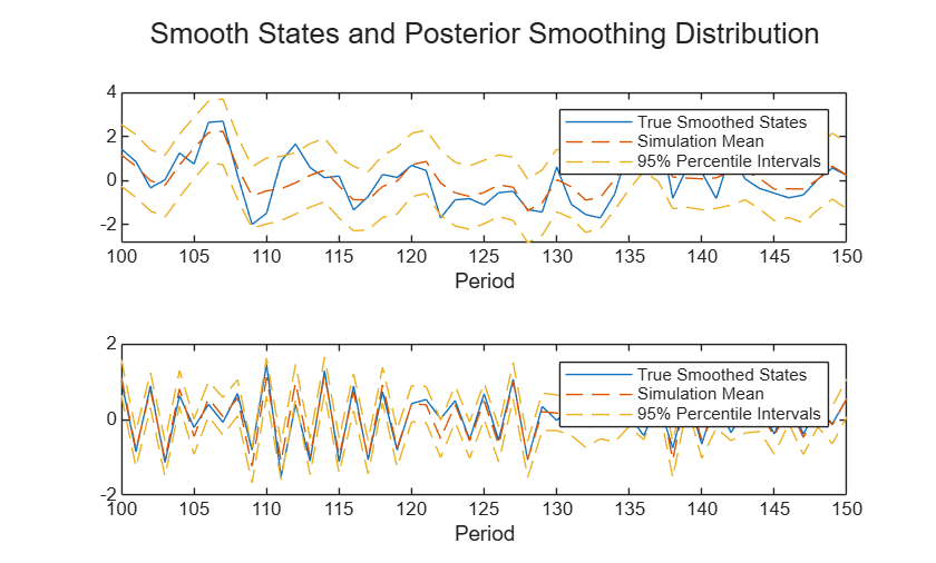
The posterior estimates are close to their associated values in the DGP.

Draw 1000 samples from the posterior state smoothing distribution, conditioned on the model parameters.

XPostSmooth = simsmooth(PriorMdl,y,estParams);

XPostSmooth is a 500-by-2-by-1000 array of the 1000 draws of the two states from the posterior state smoothing distribution, over the sampling period.

Plot the posterior state smoothing distribution means and 95% percentile intervals based on the draws. Add the true state values to the plots.

XPostSmMean = mean(XPostSmooth,3);
XPostInt = quantile(XPostSmooth,[0.025 0.975],3);

figure;
tiledlayout(2,1);
idx = (100:150);
for j = 1:width(XPostSmMean)
    nexttile
    plot(idx,X(idx,j));
    hold on
    plot(idx,XPostSmMean(idx,j),"--");
    h = plot(idx,XPostInt(idx,j,1),"--", ...
        idx,XPostInt(idx,j,2),"--");
    h(2).Color = h(1).Color;
    legend("True smoothed states","Simulation mean","95% percentile intervals");
    xlabel("Period")
end
sgtitle("Smooth States and Posterior Smoothing Distribution");

Local Functions

This example uses the following functions. paramMap is the parameter-to-matrix mapping function and priorDistribution is the log prior distribution of the parameters.

function [A,B,C,D,Mean0,Cov0,StateType] = paramMap(theta)
    A = [theta(1) 0; 0 theta(2)];
    B = [exp(theta(3)) 0; 0 exp(theta(4))]; % Map nonnegative parameters to all reals for numerical stability
    C = [1 3];
    D = 0;              % No observation noise
    Mean0 = [];         % MATLAB uses default initial state mean
    Cov0 = [];          % MATLAB uses default initial state covariances
    StateType = [0; 0]; % Two stationary states
end

function logprior = priorDistribution(theta)
    paramconstraints = [(abs(theta(1)) >= 1) (abs(theta(2)) >= 1)];
    if(sum(paramconstraints))
        logprior = -Inf;
    else 
        logprior = 0;
    end
end

Estimate Joint State Smoothing and Parameter Posterior Distribution

Open Live Script

Estimate the joint posterior state smoothing and model parameter distribution of a Bayesian state-space model, conditioned on the full data set. This example simulates observed responses from a DGP, then treats the model as Bayesian and estimates the posterior distribution of the model parameters $Θ$ and the degrees of freedom $ν_{u}$ of multivariate $t$ -distributed state disturbances.

Consider the following DGP.

$y_{t} = [\begin{array}{cccccccccccccccccccc} 1 & 3 \end{array}] [\begin{array}{cccccccccccccccccccc} x_{t, 1} \\ x_{t, 2} \end{array}] .$

The true value of the state-space parameter set $Θ = {ϕ_{1}, ϕ_{2}, σ_{1}, σ_{2}} = {0.5, - 0.75, 1, 0.5}$ .
The state disturbances $u_{1, t}$ and $u_{2, t}$ are jointly a multivariate Student's $t$ random series with $ν_{u} = 5$ degrees of freedom.

Create a vector autoregression (VAR) model that represents the state equation of the DGP.

trueTheta = [0.5; -0.75; 1; 0.5];
trueDoF = 5;
phi = [trueTheta(1) 0; 0 trueTheta(2)];
Sigma = [trueTheta(3)^2 0; 0 trueTheta(4)^2];
DGP = varm(AR={phi},Covariance=Sigma,Constant=[0; 0]);

Filter a random 2-D multivariate central $t$ series of length 500 through the VAR model to obtain the state values. Set the degrees of freedom to 5.

rng(100)  % For reproducibility
T = 500;
trueU = mvtrnd(eye(DGP.NumSeries),trueDoF,T);
X = filter(DGP,trueU);

Obtain a series of observations from the DGP by the linear combination $y_{t} = x_{1, t} + 3 x_{2, t}$ .

C = [1 3];
y = X*C';

Consider a Bayesian state-space model that represents the model with parameters $Θ$ and $ν_{u}$ treated as unknown. Assume that the joint prior distribution of the parameters in $Θ$ and $ν_{u}$ is flat but constrained to produce a stationary process.

The functions in Local Functions specify the state-space structure and prior distributions. You can use the functions only within this script.

The paramMap function accepts a vector of the unknown state-space model parameters and returns the following quantities:

A = $[\begin{array}{cc} ϕ_{1} & 0 \\ 0 & ϕ_{2} \end{array}]$ .
B = $[\begin{array}{cc} σ_{1} & 0 \\ 0 & σ_{2} \end{array}]$ .
C = $[\begin{array}{cc} 1 & 1 \end{array}]$ .
D = 0.
Mean0 and Cov0 are empty arrays [], which specify the defaults.
StateType = $[\begin{array}{cc} 0 & 0 \end{array}]$ , indicating that each state is stationary.

Create the Bayesian state-space model by passing function handles to the paramMap and priorDistribution functions to bssm. Specify that the state disturbance distribution is multivariate Student's $t$ with unknown degrees of freedom.

PriorMdl = bssm(@paramMap,@priorDistribution,StateDistribution="t");

PriorMdl is a bssm object representing the Bayesian state-space model with unknown parameters.

Estimate the posterior distribution by using estimate. Specify a random set of positive values in [0,1] to initialize the MCMC algorithm. Set the burn-in period of the MCMC algorithm to 1000 draws, and thin the entire MCMC sample by retaining every 20th draw. For numerical stability, set the univariate treatment of a multivariate model and apply the square root filter. Return the posterior estimates of the model parameters and their estimated covariance matrix.

numParamsTheta = 4;
theta0 = rand(numParamsTheta,1);
[PosteriorMdl,estParams,EstParamCov] = estimate(PriorMdl,y,theta0,Thin=20,BurnIn=1000, ...
    Univariate=true,SquareRoot=true);

Local minimum found.

Optimization completed because the size of the gradient is less than
the value of the optimality tolerance.

<stopping criteria details>
         Optimization and Tuning        
      | Params0  Optimized  ProposalStd 
----------------------------------------
 c(1) |  0.3140    0.5734      0.0832   
 c(2) |  0.7968   -0.7401      0.0372   
 c(3) |  0.8151    0.1916      0.1336   
 c(4) |  0.2625   -0.2715      0.0584   
 
               Posterior Distributions              
          |   Mean     Std   Quantile05  Quantile95 
----------------------------------------------------
 c(1)     |  0.5261  0.0786     0.3921      0.6530  
 c(2)     | -0.7602  0.0314    -0.8100     -0.7091  
 c(3)     | -0.1328  0.1336    -0.3537      0.0815  
 c(4)     | -0.6643  0.0872    -0.8069     -0.5181  
 x(1)     | -0.7516  1.0406    -2.3472      0.8641  
 x(2)     | -0.2298  0.3469    -0.7683      0.3021  
 StateDoF |  3.8793  0.7499     2.8644      5.3907  
Proposal acceptance rate = 27.37%

PosteriorMdl is a bssm object representing the posterior distribution.

Rescale state disturbance standard deviations for comparison.

exp(estParams(3:4)) % Rescale state disturbance standard deviations for comparison

ans = 2×1

    0.8756
    0.5147

The posterior estimates are close to their associated values in the DGP.

Draw 1000 samples from the joint posterior state smoothing and parameter distribution. Apply the same sampling and algorithmic options as you used earlier in the estimate function, and supply the estimated parameter covariance matrix for the Metropolis–Hastings proposal covariance.

[XPostSmooth,Parameters] = simsmooth(PriorMdl,y,estParams,Joint=true,Thin=20,BurnIn=1000, ...
    Univariate=true,SquareRoot=true,Proposal=EstParamCov);

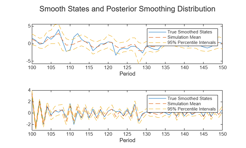
XPostSmooth is a 500-by-2-by-1000 array of the 1000 draws of the two states from the joint posterior state smoothing and parameter distribution, over the sampling period. Parameters is a 4-by-1000 matrix of the 1000 draws from the distribution.

Plot the posterior state smoothing distribution means and 95% percentile intervals based on the draws. Add the true state values to the plots.

XPostSmMean = mean(XPostSmooth,3);
XPostInt = quantile(XPostSmooth,[0.025 0.975],3);
Parameters(3:4,:) = exp(Parameters(3:4,:)); % Rescale state disturbance standard deviations

figure;
tiledlayout(2,1);
idx = (100:150);
for j = 1:width(XPostSmMean)
    nexttile
    plot(idx,X(idx,j));
    hold on;
    plot(idx,XPostSmMean(idx,j),"--");
    h = plot(idx,XPostInt(idx,j,1),"--", ...
        idx,XPostInt(idx,j,2),"--");
    h(2).Color = h(1).Color;
    legend("True smoothed states","Simulation mean","95% percentile intervals");
    xlabel("Period")
end
sgtitle("Smooth States and Posterior Smoothing Distribution");

Display trace plots of the parameter draws.

pnames = ["\phi_1" "\phi_2" "\sigma_1" "\sigma_2"];
figure
tiledlayout(2,2)
for j = 1:height(Parameters)
    nexttile
    plot(Parameters(j,:));
    title(pnames(j))
end
sgtitle("Trace Plots of Parameter Draws");

Local Functions

This example uses the following functions. paramMap is the parameter-to-matrix mapping function, and priorDistribution is the log prior distribution of the parameters.

function [A,B,C,D,Mean0,Cov0,StateType] = paramMap(theta)
    A = [theta(1) 0; 0 theta(2)];
    B = [exp(theta(3)) 0; 0 exp(theta(4))];  % Map nonnegative parameters to all reals for numerical stability
    C = [1 3];
    D = 0;              % No observation noise
    Mean0 = [];         % MATLAB uses default initial state mean
    Cov0 = [];          % MATLAB uses default initial state covariances
    StateType = [0; 0]; % Two stationary states
end

function logprior = priorDistribution(theta)
    paramconstraints = [(abs(theta(1)) >= 1) (abs(theta(2)) >= 1)];
    if(sum(paramconstraints))
        logprior = -Inf;
    else 
        logprior = 0;
    end
end

Simulate Smoothing Posterior Distribution of Regression Coefficients

Open Live Script

Model the coefficients of a linear regression as a random walk within a Bayesian state-space model, and estimate the joint posterior smoothing state and model parameter distribution.

The Bayesian state-space model is

$\begin{array}{l} y_{t} = β_{0, t} + β_{1, t} x_{1, t} + β_{2, t} x_{2, t} + u_{t} \\ β_{t} = β_{t - 1} + ε_{t}, \end{array}$

where:

$y_{t}$ is the US three-month T-bill rate.
$x_{1, t}$ is the US CPI-based inflation rate.
$x_{2, t}$ is the US M2 money supply growth rate.
$β_{t} = [\begin{array}{ccc} β_{0, t} & β_{1, t} & β_{2 t} \end{array}]'$ is the vector of coefficients.
$u_{t}$ is an iid Laplace(0, $s$ ) innovation series. The scale $s$ has a flat prior distribution.
$ε_{t}$ is a series of 3-D iid Gaussian disturbances. The variance of dimension $j$ is $σ_{j}^{2}$ and its prior distribution is $I G (2, 0.5)$ .

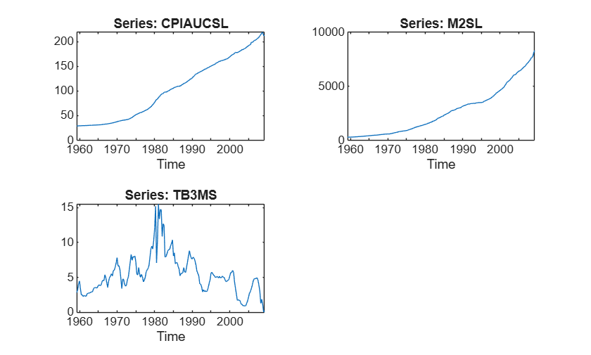
Load the US macroeconomic data Data_USEconModel.mat. The variable DataTimeTable is a timetable that contains the series in the regression model, among other series. Extract the response and predictor variables CPIAUCSL, M2SL, and TB3MS, and remove all observations that contain at least one missing value.

load Data_USEconModel
DTT = rmmissing(DataTimeTable(:,["CPIAUCSL" "M2SL" "TB3MS"]));

Plot the series separately.

figure
tiledlayout(2,2)
for j = 1:3
    nexttile
    plot(DTT.Time,DTT{:,j})
    title("Series: " + DTT.Properties.VariableNames{j})
    xlabel("Time")
end

Stabilize the series by applying the first difference to the three-month T-bill series, and by converting the predictor series to rates.

y = diff(DTT.TB3MS);
X = DTT{:,["CPIAUCSL" "M2SL"]};
X = price2ret(X)*10;

The Local Functions section contains two functions required to specify the Bayesian state-space model. You can use the functions only within this script.

The paramMap function accepts a vector of the four variances in the state-space model, the predictor data X, and the sample size $T$ , and returns the following quantities:

$A = [\begin{array}{ccc} 1 & 0 & 0 \\ 0 & 1 & 0 \\ 0 & 0 & 1 \end{array}]$ .
$B = [\begin{array}{ccc} σ_{1} & 0 & 0 \\ 0 & σ_{2} & 0 \\ 0 & 0 & σ_{3} \end{array}]$ .
$C$ is a $T$ -by-1 cell vector, where cell $t$ is $x_{t}' β_{t}$ .
$D = s$ .
Mean0 and Cov0 are empty arrays [], which specify the defaults.
StateType = $[\begin{array}{ccc} 2 & 2 & 2 \end{array}]'$ , indicating that each state is nonstationary.

Create the Bayesian state-space model by passing function handles for paramMap and priorDistribution directly to bssm. Determine the sample size $T$ , and set the values of the inverse gamma scale and shape parameters to variables.

T = numel(y);
a = 2.0; 
b = 0.5; 
PriorMdl = bssm(@(theta)paramMap(theta,X,T),@(theta)priorDistribution(theta,a,b), ...
    ObservationDistribution="Laplace");

PriorMdl is a bssm object representing the Bayesian state-space model.

Fit the model to the data. Choose the initial states of the state disturbance standard deviations randomly from $I G (2, 0.5)$ , and set the initial state of the Laplace scale to 1. Reduce transient effects and serial correlation in the sample by setting a burn-in period of 1000 and a thinning factor of 20. Because the observation innovations are uncorrelated, set the univariate treatment of the multivariate model for computational efficiency. For numerical stability, apply the square root filter. Return the posterior estimates of the model parameters and their estimated covariance matrix.

rng(1,"twister")
params0 = [1./gamrnd(a,b,3,1); 1]; 
[PosteriorMdl,estParams,EstParamCov] = estimate(PriorMdl,y,params0,Thin=20,BurnIn=1000, ...
    Univariate=true,SquareRoot=true);

Local minimum possible.

fminunc stopped because the size of the current step is less than
the value of the step size tolerance.

<stopping criteria details>
         Optimization and Tuning        
      | Params0  Optimized  ProposalStd 
----------------------------------------
 c(1) |  0.5400    0.0854      0.0273   
 c(2) |  5.5331    6.5892      1.0647   
 c(3) |  3.3037    0.1669      0.0850   
 c(4) |   1        0.4659      0.0594

             Posterior Distributions            
      |   Mean     Std   Quantile05  Quantile95 
------------------------------------------------
 c(1) |  0.0982  0.0321     0.0537      0.1537  
 c(2) |  0.2894  0.2013     0.0910      0.7066  
 c(3) |  0.2143  0.1127     0.0864      0.4373  
 c(4) |  0.5565  0.0441     0.4915      0.6321  
 x(1) |  0.1526  0.3641    -0.4710      0.7430  
 x(2) |  1.1180  1.4362    -1.2977      3.3429  
 x(3) | -2.2551  1.4254    -4.6804     -0.0432  
Proposal acceptance rate = 7.58%

PosteriorMdl is a bssm object representing the posterior distribution.

Obtain posterior estimates from the joint posterior smoothing distribution of the regression coefficients and the model parameters. Apply the same sampling and algorithmic options as you used earlier for the estimate function, and supply the estimated parameter covariance matrix for the Metropolis–Hastings proposal covariance.

[BetaPostSmooth,Parameters] = simsmooth(PriorMdl,y,estParams,Joint=true, ...
    Proposal=EstParamCov,Thin=20,BurnIn=1000,Univariate=true,Squareroot=true);

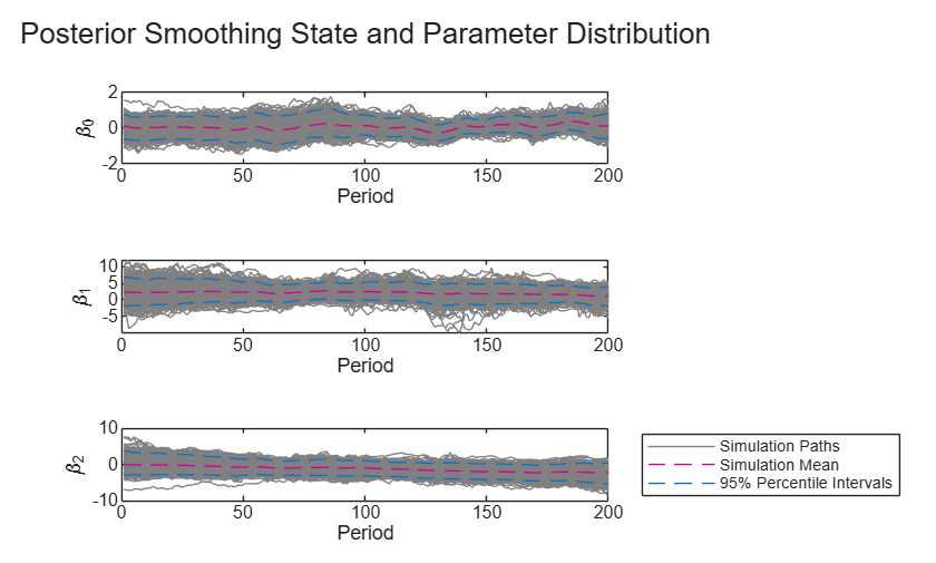
BetaPostSmooth is a T-by-3-by-1000 array of the 1000 draws of the three regression coefficients from the joint posterior state smoothing and parameter distribution, over the sampling period. Parameters is a 4-by-1000 matrix of the 1000 draws from the distribution.

Plot the posterior state smoothing distribution means and 95% percentile intervals based on the draws.

BetaPostSmMean = mean(BetaPostSmooth,3);
BetaPostInt = quantile(BetaPostSmooth,[0.025 0.975],3);

figure;
p = width(BetaPostSmMean);
tiledlayout(p,1);
idx = 1:T;
for j = 1:p
    nexttile
    h1 = plot(idx,squeeze(BetaPostSmooth(idx,j,:)),Color=[0.5 0.5 0.5]);
    hold on;
    h2 = plot(idx,BetaPostSmMean(idx,j),"--");
    h3 = plot(idx,BetaPostInt(idx,j,1),"--", ...
        idx,BetaPostInt(idx,j,2),"--");
    h3(2).Color = h3(1).Color;
    ylabel("\beta_" + string(j-1))
    xlabel("Period")
end
legend([h1(1) h2 h3(1)],["Simulation paths" "Simulation mean" "95% percentile intervals"], ...
    Location="eastoutside");
sgtitle("Posterior Smoothing State and Parameter Distribution");

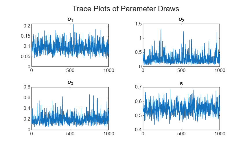
Display trace plots of the parameter draws.

pnames = ["\sigma_1" "\sigma_2" "\sigma_3" "s"];
figure
tiledlayout("flow")
for j = 1:height(Parameters)
    nexttile
    plot(Parameters(j,:));
    title(pnames(j))
end
sgtitle("Trace Plots of Parameter Draws");

Local Functions

This example uses the following functions. paramMap is the parameter-to-matrix mapping function, and priorDistribution is the log prior distribution of the parameters.

function [A,B,C,D,Mean0,Cov0,StateType] = paramMap(theta,Z,T)
A = eye(3);
B = diag(theta(1:3));
C = cell(T,1);
for t = 1:T
    C{t} = [1 Z(t,:)];
end
D = theta(4);          % Laplace scale s
Mean0 = [];            % MATLAB uses default initial state mean
Cov0 = [];             % MATLAB uses default initial state covariances
StateType = [2; 2; 2]; % Three nonstationary states
end

function logprior = priorDistribution(theta,a,b)
paramconstraints = theta < 0;
if(sum(paramconstraints))
    logprior = -Inf;
else 
    p = zeros(3,1);
    for j = 1:numel(p)
        p(j) = a*log(b) - gammaln(a) - (a+1)*log(theta(j)) - b./theta(j);
    end
    logprior = sum(p);
end
end

Input Arguments

collapse all

`PriorMdl` — Prior Bayesian linear state-space model
`bssm` model object

Prior Bayesian linear state-space model, specified as a bssm model object returned by bssm or ssm2bssm.

The function handles of the properties PriorMdl.ParamDistribution and PriorMdl.ParamMap determine the prior distribution and the data likelihood, respectively. simsmooth evaluates PriorMdl.ParamMap at params before computing the posterior smoothing state distribution.

`Y` — Observed response data
numeric matrix | cell vector of numeric vectors

Observed response data, from which simsmooth forms the posterior distribution, specified as a numeric matrix or a cell vector of numeric vectors.

If PriorMdl is time invariant with respect to the observation equation, Y is a T-by-n matrix. Each row of the matrix corresponds to a period, and each column corresponds to a particular observation in the model. T is the sample size and n is the number of observations per period. The last row of Y contains the latest observations.
If PriorMdl is time varying with respect to the observation equation, Y is a T-by-1 cell vector. Y{t} contains an n_t-dimensional vector of observations for period t, where t = 1, ..., T. The corresponding dimensions of the coefficient matrices, outputs of PriorMdl.ParamMap, C{t}, and D{t} must be consistent with the matrix in Y{t} for all periods. The last cell of Y contains the latest observations.

NaN elements indicate missing observations. For details on how the Kalman filter accommodates missing observations, see Algorithms.

Data Types: double | cell

`params` — State-space model parameters Θ
numeric vector

State-space model parameters Θ used to evaluate the parameter mapping Mdl.ParamMap, specified as a numparams-by-1 numeric vector. Elements of params must correspond to the elements of the first input arguments of PriorMdl.ParamMap and PriorMdl.ParamDistribution.

Usually, you pass either the posterior means of the parameters or a draw from their posterior distribution to params. The second output of estimate contains the posterior means of the parameters, and the first output of simulate contains draws from their posterior distribution.

Data Types: double

Name-Value Arguments

expand all

Specify optional pairs of arguments as Name1=Value1,...,NameN=ValueN, where Name is the argument name and Value is the corresponding value. Name-value arguments must appear after other arguments, but the order of the pairs does not matter.

Example: simsmooth(PriorMdl,Y,params,NumDraws=1e4,Joint=true) specifies to generate 1e4 random draws from the posterior, and to sample from the joint posterior distribution of the smoothed states and state-space model parameters.

Options for All Situations

expand all

`Joint` — Flag for sampling from joint posterior distribution
`false` (default) | `true`

Flag for sampling from the joint posterior distribution of the states and model parameters, specified as false or true.

Value Description

Value	Description
`false`	`simsmooth` samples from the posterior smoothing distribution evaluated at Θ = `params`, p(x_T,…,x₀\|y_T,…,y₁,Θ). `simsmooth` applies forward-filtering, backward-smoothing of the standard view of the state-space model. `simsmooth` does not account for parameter uncertainty when estimating the state smoothing posterior distribution.
`true`	`simsmooth` samples from the joint posterior smoothing and model parameter distribution p(x_T,…,x₀,Θ\|y_T,…,y₁) by implementing the forward-filtering, backward-sampling method. `simsmooth` uses the Metropolis–Within–Gibbs sampler to sample from the joint posterior smoothing distribution, and initializes the sampler using `params`. `simsmooth` accounts for parameter uncertainty when estimating the state smoothing posterior distribution.

false

simsmooth samples from the posterior smoothing distribution evaluated at Θ = params, p(x_T,…,x₀|y_T,…,y₁,Θ).

simsmooth applies forward-filtering, backward-smoothing of the standard view of the state-space model.
simsmooth does not account for parameter uncertainty when estimating the state smoothing posterior distribution.

true

simsmooth samples from the joint posterior smoothing and model parameter distribution p(x_T,…,x₀,Θ|y_T,…,y₁) by implementing the forward-filtering, backward-sampling method.

simsmooth uses the Metropolis–Within–Gibbs sampler to sample from the joint posterior smoothing distribution, and initializes the sampler using params.
simsmooth accounts for parameter uncertainty when estimating the state smoothing posterior distribution.

Example: Joint=true

Data Types: logical

`NumDraws` — Number of posterior sample draws
`1000` (default) | positive integer

Number of posterior sample draws, specified as a positive integer.

Example: NumDraws=1e5

Data Types: double

Metropolis–Hastings Sampler Options When `Joint=true`

expand all

`BurnIn` — Number of draws to remove from beginning of sample
`100` (default) | nonnegative scalar

Number of draws to remove from the beginning of the sample to reduce transient effects, specified as a nonnegative scalar. For details on how simsmooth reduces the full sample, see Algorithms.

Tip

To help you specify the appropriate burn-in period size:

Determine the extent of the transient behavior in the sample by setting the BurnIn name-value argument to 0.
Simulate a few thousand observations by using simulate.
Create trace plots.

Example: BurnIn=1000

Data Types: double

`Thin` — Adjusted sample size multiplier
`1` (no thinning) (default) | positive integer

Adjusted sample size multiplier, specified as a positive integer.

The actual sample size is BurnIn + NumDraws*Thin. After discarding the burn-in, simsmooth discards every Thin – 1 draws, and then retains the next draw. For more details on how simsmooth reduces the full sample, see Algorithms.

Tip

To reduce potential large serial correlation in the posterior sample, or to reduce the memory consumption of the output sample, specify a large value for Thin, such as 15.

Example: Thin=5

Data Types: double

`Univariate` — Flag for univariate treatment of multivariate series
`false` (default) | `true`

Flag for the univariate treatment of a multivariate series, specified as false or true.

Value	Description
`true`	Applies the univariate treatment of a multivariate series, also known as sequential filtering
`false`	Does not apply sequential filtering

The univariate treatment can accelerate and improve numerical stability of the Kalman filter. However, all observation innovations must be uncorrelated. That is, D_tD_t' must be diagonal, where D_t (t = 1, ..., T) is the output coefficient matrix D of PriorMdl.ParamMap.

Example: Univariate=true

Data Types: logical

`SquareRoot` — Flag for square root filter method
`false` (default) | `true`

Flag for the square root filter method, specified as false or true.

Value	Description
`true`	Applies the square root filter method for the Kalman filter
`false`	Does not apply the square root filter method

If you think the eigenvalues of the filtered state or forecasted observation covariance matrices are close to zero, then specify SquareRoot=true. The square root filter is robust to numerical issues arising from the finite precision of calculations, but requires more computational resources.

Example: SquareRoot=true

Data Types: logical

`DoF` — Proposal distribution degrees of freedom
`Inf` (default) | positive scalar

Proposal distribution degrees of freedom for parameter updates made using the Metropolis–Hastings (MH) sampler, specified as Inf or a positive scalar.

Value	MH Proposal Distribution
Positive scalar	Multivariate t with `DoF` degrees of freedom
`Inf`	Multivariate normal

Example: DoF=10

Data Types: double

`Proposal` — MH proposal distribution scale (covariance) matrix for parameters Θ
positive definite numeric matrix

MH proposal distribution scale (covariance) matrix for the parameters Θ, up to the proportionality constant Proportion, specified as a numParams-by-numParams positive definite numeric matrix. Elements of Proposal must correspond to elements in params.

The proposal distribution is multivariate normal or Student's t with DoF degrees of freedom (for details, see DoF).

By default, simsmooth uses tune to obtain a proposal scale matrix. This action increases execution time.

Data Types: double

`Proportion` — Proportionality constant
`1` (default) | positive scalar

Proportionality constant of the proposal scale matrix, specified as a positive scalar.

Tip

For higher proposal acceptance rates, experiment with relatively small values for Proportion, such as 0.1.

Example: Proportion=1

Data Types: double

`Center` — Proposal distribution center
`[]` (default) | numeric vector

Proposal distribution center, specified as numParams-by-1 numeric vector.

simsmooth uses the independence MH sampler, and Center is the center of the proposal distribution.

When Center is an empty array [] (the default), simsmooth uses the random-walk MH sampler. The center of the proposal distribution is the current state of the Markov chain.

Example: Center=ones(10,1)

Data Types: double

`Hessian` — Hessian approximation method
`"difference"` (default) | `"diagonal"` | `"opg"` | `"optimizer"` | character vector

Hessian approximation method for the MH proposal distribution scale matrix, specified as a value in this table.

Value	Description
`"difference"`	Finite differencing
`"diagonal"`	Diagonalized result of finite differencing
`"opg"`	Outer product of gradients, ignoring the prior distribution
`"optimizer"`	Posterior distribution optimized by `fmincon` or `fminunc`. Specify optimization options by using the `Options` name-value argument.

Tip

The Hessian="difference" setting can be computationally intensive and inaccurate, and the resulting scale matrix might not be positive definite. Try one of the other options for better results.

Example: Hessian="opg"

Data Types: char | string

`Lower` — Parameter lower bounds
`[]` (default) | numeric vector

Parameter lower bounds for computing the Hessian matrix (see Hessian), specified as a numParams-by-1 numeric vector.

Lower(j) specifies the lower bound of parameter theta(j), the first input argument of the functions represented in PriorMdl.ParamMap and PriorMdl.ParamDistribution.

The default value [] specifies no lower bounds.

Note

Lower does not apply to posterior simulation. To apply parameter constraints on the posterior, code them in the log prior distribution function PriorMdl.ParamDistribution by setting the log prior to -Inf for values outside the distribution support.

Example: Lower=[0 -5 -1e7]

Data Types: double

`Upper` — Parameter upper bounds
`[]` (default) | numeric vector

Parameter upper bounds for computing the Hessian matrix (see Hessian), specified as a numParams-by-1 numeric vector.

Upper(j) specifies the upper bound of parameter theta(j), the first input argument of the functions represented in PriorMdl.ParamMap and PriorMdl.ParamDistribution.

The default value [] specifies no upper bounds.

Note

Upper does not apply to posterior simulation. To apply parameter constraints on the posterior, code them in the log prior distribution function PriorMdl.ParamDistribution by setting the log prior to -Inf for values outside the distribution support.

Example: Upper=[5 100 1e7]

Data Types: double

`Options` — Optimization options
`optimoptions` optimization controller

Optimization options for the setting Hessian="optimizer", specified as an optimoptions optimization controller. Options replaces the default optimization options of the optimizer. For details on changing the default values of the optimizer, see the optimization controller optimoptions, the constrained optimization function fmincon, or the unconstrained optimization function fminunc in Optimization Toolbox™.

By default, simsmooth uses the default options of the optimizer.

Example: To change the constraint tolerance to 1e-6, set options = optimoptions(@fmincon,ConstraintTolerance=1e-6,Algorithm="sqp"). Then, pass Options by using Options=options.

`Simplex` — Simplex search flag
`true` (default) | `false`

Simplex search flag to improve the initial parameter values, specified as true or faase.

Value	Description
`true`	Applies the simplex search method to improve the initial parameter values for proposal optimization. For more details, see fminsearch Algorithm.
`false`	Does not apply the simplex search method

simsmooth applies the simplex search when the numerical optimization exit flag is not positive.

Example: Simplex=false

Data Types: logical

`Display` — Flag for displaying proposal tuning results
`true` (default) | `false`

Flag for displaying proposal tuning results , specified as a value in this table.

Value	Description
`true`	Displays the tuning results
`false`	Does not display the tuning results

Example: Display=false

Data Types: logical

`StdDoF` — Proposal standard deviation for degrees of freedom parameter
`0.1` (default) | positive numeric scalar

Proposal standard deviation for the degrees of freedom parameter of the t-distributed state disturbance or observation innovation process, specified as a positive numeric scalar.

StdDoF applies to the corresponding process when PriorMdl.StateDistribution.Name is "t" or PriorMdl.ObservationDistribution.Name is "t", and their associated degrees of freedom are estimable (the DoF field is NaN or a function handle). For example, if the following conditions hold, StdDof applies only to the t-distribution degrees of freedom of the state disturbance process:

PriorMdl.StateDistribution.Name is "t".
PriorMdl.StateDistribution.DoF is NaN.
The limiting distribution of the observation innovations is Gaussian (PriorMdl.ObservationDistribution.Name is "Gaussian" or PriorMdl.ObservationDistribution is struct("Name","t","DoF",Inf)).

Example: StdDoF=0.5

Data Types: double

Output Arguments

collapse all

`X` — Simulated paths of smoothed states
numeric matrix | 3-D numeric array | cell vector of numeric matrices

Simulated paths of the smoothed states, drawn from the posterior smoothed state distribution p(x_T,…,x₀|y_T,…,y₁,Θ) for t = 1,…,T, returned as a T-by-m numeric matrix for one simulated path, a T-by-m-by-NumDraws 3-D numeric array for NumDraws simulated paths, or a T-by-1 cell vector of numeric matrices.

Each row corresponds to a time point in the sample. The last row contains the latest simulated smoothed states.

If PriorMdl is time-invariant with respect to the states, each column of X corresponds to a state in the model, and each page corresponds to a sample path.

If PriorMdl is time varying with respect to the states, for each t = 1,…,T, cell X(t) contains an m_t-by-NumDraws matrix of simulated smoothed states. Each row corresponds to a state variable for the corresponding time, and each column corresponds to a simulated path. For each k, column k of the matrices across all cells contains the state path of draw k.

`Parameters` — Posterior draws
numeric matrix

Posterior draws of the state-space model parameters Θ, returned as a numParams-by-NumDraws numeric matrix. Each column is a separate draw from the distribution. Each row corresponds to the corresponding element of params.

Because the Metropolis–Within–Gibbs sampler is a Markov chain, successive draws are correlated.

Algorithms

The functionality of the simulation smoother simsmooth depends on the value of Joint.

When Joint is false, simsmooth applies the conditional mean adjustment simulation smoother [2] to simulate state paths from the posterior smoothing distribution conditioned on the parameters. simsmooth treats PriorMdl as non-Bayesian and dispatches the state-space model to the simsmooth function of the ssm object.
When Joint is true, simsmooth applies the Metropolis–within–Gibbs sampler[1] to simulate smoothing states and model parameters from their joint posterior distribution by using this procedure:
1. Obtain a proposal covariance by tuning the sampler (tune).
2. Simulate states and model parameters from the joint posterior using the MCMC method (simulate).

The Kalman filter accommodates missing data by not updating the filtered state estimates that correspond to missing observations. In other words, assume a missing observation at period t. The state forecast for period t based on the previous t – 1 observations is equivalent to the filtered state for period t.

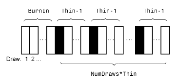
The figure below shows how simsmooth reduces the sample by using the values of NumDraws, Thin, and BurnIn. Rectangles represent successive draws from the distribution. simsmooth removes the white rectangles from the sample. The remaining NumDraws black rectangles compose the sample.

Sample reduced by using the values of NumDraws, Thin, and BurnIn

References

[1] Doucet, Arnaud, Simon Godsill, and Christophe Andrieu. "On Sequential Monte Carlo Sampling Methods for Bayesian Filtering." Statistics and Computing 10 (July 2000): 197–208. https://doi.org/10.1023/A:1008935410038.

[2] Durbin, J., and Siem Jan Koopman. Time Series Analysis by State Space Methods. 2nd ed. Oxford: Oxford University Press, 2012.

[3] Hastings, Wilfred K. "Monte Carlo Sampling Methods Using Markov Chains and Their Applications." Biometrika 57 (April 1970): 97–109. https://doi.org/10.1093/biomet/57.1.97.

[4] Metropolis, Nicholas, Arianna. W. Rosenbluth, Marshall. N. Rosenbluth, Augusta. H. Teller, and Edward Teller. "Equation of State Calculations by Fast Computing Machines." The Journal of Chemical Physics 21 (June 1953): 1087–92. https://doi.org/10.1063/1.1699114.

Version History

Introduced in R2026b

simsmooth

Syntax

Description

Examples

Estimate Posterior Smoothing Conditional Distribution

Estimate Joint State Smoothing and Parameter Posterior Distribution

Simulate Smoothing Posterior Distribution of Regression Coefficients

Input Arguments

`PriorMdl` — Prior Bayesian linear state-space model
`bssm` model object

`Y` — Observed response data
numeric matrix | cell vector of numeric vectors

`params` — State-space model parameters Θ
numeric vector

Name-Value Arguments

Options for All Situations

`Joint` — Flag for sampling from joint posterior distribution
`false` (default) | `true`

`NumDraws` — Number of posterior sample draws
`1000` (default) | positive integer

Metropolis–Hastings Sampler Options When `Joint=true`

`BurnIn` — Number of draws to remove from beginning of sample
`100` (default) | nonnegative scalar

`Thin` — Adjusted sample size multiplier
`1` (no thinning) (default) | positive integer

`Univariate` — Flag for univariate treatment of multivariate series
`false` (default) | `true`

`SquareRoot` — Flag for square root filter method
`false` (default) | `true`

`DoF` — Proposal distribution degrees of freedom
`Inf` (default) | positive scalar

`Proposal` — MH proposal distribution scale (covariance) matrix for parameters Θ
positive definite numeric matrix

`Proportion` — Proportionality constant
`1` (default) | positive scalar

`Center` — Proposal distribution center
`[]` (default) | numeric vector

`Hessian` — Hessian approximation method
`"difference"` (default) | `"diagonal"` | `"opg"` | `"optimizer"` | character vector

`Lower` — Parameter lower bounds
`[]` (default) | numeric vector

`Upper` — Parameter upper bounds
`[]` (default) | numeric vector

`Options` — Optimization options
`optimoptions` optimization controller

`Simplex` — Simplex search flag
`true` (default) | `false`

`Display` — Flag for displaying proposal tuning results
`true` (default) | `false`

`StdDoF` — Proposal standard deviation for degrees of freedom parameter
`0.1` (default) | positive numeric scalar

Output Arguments

`X` — Simulated paths of smoothed states
numeric matrix | 3-D numeric array | cell vector of numeric matrices

`Parameters` — Posterior draws
numeric matrix

Algorithms

References

Version History

See Also

Objects

Functions

simsmooth

Syntax

Description

Examples

Estimate Posterior Smoothing Conditional Distribution

Estimate Joint State Smoothing and Parameter Posterior Distribution

Simulate Smoothing Posterior Distribution of Regression Coefficients

Input Arguments

PriorMdl — Prior Bayesian linear state-space model bssm model object

Y — Observed response data numeric matrix | cell vector of numeric vectors

params — State-space model parameters Θ numeric vector

Name-Value Arguments

Options for All Situations

Joint — Flag for sampling from joint posterior distribution false (default) | true

NumDraws — Number of posterior sample draws 1000 (default) | positive integer

Metropolis–Hastings Sampler Options When Joint=true

BurnIn — Number of draws to remove from beginning of sample 100 (default) | nonnegative scalar

Thin — Adjusted sample size multiplier 1 (no thinning) (default) | positive integer

Univariate — Flag for univariate treatment of multivariate series false (default) | true

SquareRoot — Flag for square root filter method false (default) | true

DoF — Proposal distribution degrees of freedom Inf (default) | positive scalar

Proposal — MH proposal distribution scale (covariance) matrix for parameters Θ positive definite numeric matrix

Proportion — Proportionality constant 1 (default) | positive scalar

Center — Proposal distribution center [] (default) | numeric vector

Hessian — Hessian approximation method "difference" (default) | "diagonal" | "opg" | "optimizer" | character vector

Lower — Parameter lower bounds [] (default) | numeric vector

Upper — Parameter upper bounds [] (default) | numeric vector

Options — Optimization options optimoptions optimization controller

Simplex — Simplex search flag true (default) | false

Display — Flag for displaying proposal tuning results true (default) | false

StdDoF — Proposal standard deviation for degrees of freedom parameter 0.1 (default) | positive numeric scalar

Output Arguments

X — Simulated paths of smoothed states numeric matrix | 3-D numeric array | cell vector of numeric matrices

Parameters — Posterior draws numeric matrix

Algorithms

References

Version History

See Also

Objects

Functions

`PriorMdl` — Prior Bayesian linear state-space model
`bssm` model object

`Y` — Observed response data
numeric matrix | cell vector of numeric vectors

`params` — State-space model parameters Θ
numeric vector

`Joint` — Flag for sampling from joint posterior distribution
`false` (default) | `true`

`NumDraws` — Number of posterior sample draws
`1000` (default) | positive integer

Metropolis–Hastings Sampler Options When `Joint=true`

`BurnIn` — Number of draws to remove from beginning of sample
`100` (default) | nonnegative scalar

`Thin` — Adjusted sample size multiplier
`1` (no thinning) (default) | positive integer

`Univariate` — Flag for univariate treatment of multivariate series
`false` (default) | `true`

`SquareRoot` — Flag for square root filter method
`false` (default) | `true`

`DoF` — Proposal distribution degrees of freedom
`Inf` (default) | positive scalar

`Proposal` — MH proposal distribution scale (covariance) matrix for parameters Θ
positive definite numeric matrix

`Proportion` — Proportionality constant
`1` (default) | positive scalar

`Center` — Proposal distribution center
`[]` (default) | numeric vector

`Hessian` — Hessian approximation method
`"difference"` (default) | `"diagonal"` | `"opg"` | `"optimizer"` | character vector

`Lower` — Parameter lower bounds
`[]` (default) | numeric vector

`Upper` — Parameter upper bounds
`[]` (default) | numeric vector

`Options` — Optimization options
`optimoptions` optimization controller

`Simplex` — Simplex search flag
`true` (default) | `false`

`Display` — Flag for displaying proposal tuning results
`true` (default) | `false`

`StdDoF` — Proposal standard deviation for degrees of freedom parameter
`0.1` (default) | positive numeric scalar

`X` — Simulated paths of smoothed states
numeric matrix | 3-D numeric array | cell vector of numeric matrices

`Parameters` — Posterior draws
numeric matrix