checkGradients
语法
说明
除了前面语法中的任何输入参量组合之外,valid = checkGradients(___,Name=Value)
示例
本例末尾的 rosen 函数计算二维变量 x 的 Rosenbrock 目标函数及其梯度。
检查 rosen 中计算的梯度是否与点 [2,4] 附近的有限差分近似相匹配。
x0 = [2,4];
valid = checkGradients(@rosen,x0)
valid = logical
   1
function [f,g] = rosen(x)
f = 100*(x(1) - x(2)^2)^2 + (1 - x(2))^2;
if nargout > 1
    g(1) = 200*(x(1) - x(2)^2);
    g(2) = -400*x(2)*(x(1) - x(2)^2) - 2*(1 - x(2));
end
end
本例末尾的 vecrosen 函数以最小二乘形式计算 Rosenbrock 目标函数及其雅可比矩阵(梯度)。
检查 vecrosen 中计算的梯度是否与点 [2,4] 附近的有限差分近似相匹配。
x0 = [2,4];
valid = checkGradients(@vecrosen,x0)
valid = logical
   1
function [f,g] = vecrosen(x)
f = [10*(x(1) - x(2)^2),1-x(1)];
if nargout > 1
    g = zeros(2); % Allocate g
    g(1,1) = 10; % df(1)/dx(1)
    g(1,2) = -20*x(2); % df(1)/dx(2)
    g(2,1) = -1; % df(2)/dx(1)
    g(2,2) = 0; % df(2)/dx(2)
end
end
本例末尾的 rosen 函数计算二维变量 x 的 Rosenbrock 目标函数及其梯度。
对于一些初始点,默认的正向有限差分导致 checkGradients 错误地指示 rosen 函数具有不正确的梯度。要查看结果详情,请将 Display 选项设置为 "on"。
x0 = [0,0];
valid = checkGradients(@rosen,x0,Display="on")
____________________________________________________________ Objective function derivatives: Maximum relative difference between supplied and finite-difference derivatives = 1.48826e-06. Supplied derivative element (1,1): -0.126021 Finite-difference derivative element (1,1): -0.126023 checkGradients failed. Supplied derivative and finite-difference approximation are not within 'Tolerance' (1e-06). ____________________________________________________________
valid = logical
   0
checkGradients 报告不匹配,小数点后第六位相差刚好超过 1。使用中心有限差分并再次检查。
opts = optimoptions("fmincon",FiniteDifferenceType="central");
valid = checkGradients(@rosen,x0,opts,Display="on")
____________________________________________________________

Objective function derivatives:
Maximum relative difference between supplied
and finite-difference derivatives = 1.29339e-11.

checkGradients successfully passed.
____________________________________________________________
valid = logical
   1
中心有限差分通常更准确。checkGradients 报告称梯度和中心有限差分近似匹配到小数点后约 11 位。
function [f,g] = rosen(x)
f = 100*(x(1) - x(2)^2)^2 + (1 - x(2))^2;
if nargout > 1
    g(1) = 200*(x(1) - x(2)^2);
    g(2) = -400*x(2)*(x(1) - x(2)^2) - 2*(1 - x(2));
end
end
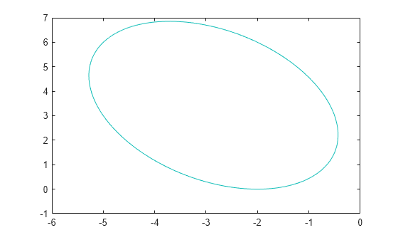
此示例末尾的 tiltellipse 函数施加了约束,即二维变量 x 被限制在倾斜椭圆的内部
.
将椭圆可视化。
f = @(x,y) x.*y/2+(x+2).^2+(y-2).^2/2-2;
fcontour(f,LevelList=0)
axis([-6 0 -1 7])
检查这个非线性不等式约束函数的梯度。
x0 = [-2,6];
valid = checkGradients(@tiltellipse,x0,IsConstraint=true)
valid = 1×2 logical array

   1   1
function [c,ceq,gc,gceq] = tiltellipse(x)
c = x(1)*x(2)/2 + (x(1) + 2)^2 + (x(2)- 2)^2/2 - 2;
ceq = [];

if nargout > 2
   gc = [x(2)/2 + 2*(x(1) + 2);
       x(1)/2 + x(2) - 2];
   gceq = [];
end
end
此示例末尾的 fungrad 函数正确计算了最小二乘目标某些分量的梯度,但错误地计算了其他成分的梯度。
检查 checkGradients 的第二个输出,查看哪些分量在点 [2,4] 处匹配不太好。要查看结果详情,请将 Display 选项设置为 "on"。
x0 = [2,4];
[valid,err] = checkGradients(@fungrad,x0,Display="on")
____________________________________________________________ Objective function derivatives: Maximum relative difference between supplied and finite-difference derivatives = 0.749797. Supplied derivative element (3,2): 19.9838 Finite-difference derivative element (3,2): 5 checkGradients failed. Supplied derivative and finite-difference approximation are not within 'Tolerance' (1e-06). ____________________________________________________________
valid = logical
   0
err = struct with fields:
    Objective: [3×2 double]
输出表明元素 [3,2] 不正确。但这是唯一的问题吗?检查 err.Objective 并查找远离 0 的条目。
err.Objective
ans = 3×2

    0.0000    0.0000
    0.0000         0
    0.5000    0.7498
导数的 [3,1] 和 [3,2] 元素都是不正确的。本示例末尾的 fungrad2 函数可纠正错误。
[valid,err] = checkGradients(@fungrad2,x0,Display="on")____________________________________________________________ Objective function derivatives: Maximum relative difference between supplied and finite-difference derivatives = 2.2338e-08. checkGradients successfully passed. ____________________________________________________________
valid = logical
   1
err = struct with fields:
    Objective: [3×2 double]
err.Objective
ans = 3×2
10-7 ×

    0.2234    0.0509
    0.0003         0
    0.0981    0.0042
梯度近似和有限差分近似之间的所有差异在数量级上均小于 1e-7。
以下代码创建 fungrad 辅助函数。
function [f,g] = fungrad(x)
f = [10*(x(1) - x(2)^2),1 - x(1),5*(x(2) - x(1)^2)];

if nargout > 1
    g = zeros(3,2);
    g(1,1) = 10;
    g(1,2) = -20*x(2);
    g(2,1) = -1;
    g(3,1) = -20*x(1);
    g(3,2) = 5*x(2);
end
end
以下代码创建 fungrad2 辅助函数。
function [f,g] = fungrad2(x)
f = [10*(x(1) - x(2)^2),1 - x(1),5*(x(2) - x(1)^2)];

if nargout > 1
    g = zeros(3,2);
    g(1,1) = 10;
    g(1,2) = -20*x(2);
    g(2,1) = -1;
    g(3,1) = -10*x(1);
    g(3,2) = 5;
end
end
当您提供梯度计算函数时,非线性最小二乘求解器(如 lsqcurvefit)可以更快、更可靠地运行。然而,与其它求解器相比,lsqcurvefit 求解器在检查梯度时语法略有不同。
拟合问题和 checkGradient 语法
要检查 lsqcurvefit 梯度,不要将初始点 x0 作为数组传递,而是传递元胞数组 {x0,xdata}。例如,对于响应函数 ,从模型中创建添加了噪声的数据 ydata。响应函数为 fitfun。
function [F,J] = fitfun(x,xdata)
F = x(1) + x(2)*exp(-x(3)*xdata);
if nargout > 1
    J = [ones(size(xdata)) exp(-x(3)*xdata) -xdata.*x(2).*exp(-x(3)*xdata)];
end
end
生成 xdata 作为从 0 到 10 的随机点,并将 ydata 作为响应加上添加的噪声。
a = 2;
b = 5;
c = 1/15;
N = 100;
rng default
xdata = 10*rand(N,1);
fun = @fitfun;
ydata = fun([a,b,c],xdata) + randn(N,1)/10;
检查响应函数在点 [a,b,c] 的梯度是否正确。
[valid,err] = checkGradients(@fitfun,{[a b c] xdata})valid = logical
1
err = struct with fields:
    Objective: [100×3 double]
您可以安全地使用提供的目标梯度。将所有参数的下界设置为 0,无上界。
options = optimoptions("lsqcurvefit",SpecifyObjectiveGradient=true);
lb = zeros(1,3);
ub = [];
[sol,res,~,eflag,output] = lsqcurvefit(fun,[1 2 1],xdata,ydata,lb,ub,options)
Local minimum possible. lsqcurvefit stopped because the final change in the sum of squares relative to its initial value is less than the value of the function tolerance. <stopping criteria details>
sol = 1×3

    2.5872    4.4376    0.0802
res =
1.0096
eflag =
3
output = struct with fields:
      firstorderopt: 4.4156e-06
         iterations: 25
          funcCount: 26
       cgiterations: 0
          algorithm: 'trust-region-reflective'
           stepsize: 1.8029e-04
            message: 'Local minimum possible.↵↵lsqcurvefit stopped because the final change in the sum of squares relative to ↵its initial value is less than the value of the function tolerance.↵↵<stopping criteria details>↵↵Optimization stopped because the relative sum of squares (r) is changing↵by less than options.FunctionTolerance = 1.000000e-06.'
       bestfeasible: []
    constrviolation: []
lsqcurvefit 中的非线性约束函数
非线性约束函数所需的语法与 lsqcurvefit 目标函数的语法不同。具有梯度的非线性约束函数具有以下形式:
function [c,ceq,gc,gceq] = ccon(x)
c = ...
ceq = ...
if nargout > 2
    gc = ...
    gceq = ...
end
end
梯度表达式的大小必须为 NxNc,其中 N 是问题变量的数量,Nc 是约束函数的数量。例如,下面的 ccon 函数只有一个非线性不等式约束。因此,对于这个包含三个变量的方程,该函数返回一个 3×1 的梯度。
function [c,ceq,gc,gceq] = ccon(x)
ceq = [];
c = x(1)^2 + x(2)^2 + 1/x(3)^2 - 50;
if nargout > 2
    gceq = [];
    gc = zeros(3,1); % Gradient is a column vector
    gc(1) = 2*x(1);
    gc(2) = 2*x(2);
    gc(3) = -2/x(3)^3;
end
end
检查函数 ccon 在点 [a,b,c] 返回的梯度是否正确。
[valid,err] = checkGradients(@ccon,[a b c],IsConstraint=true)
valid = 1×2 logical array

   1   1
err = struct with fields:
    Inequality: [3×1 double]
      Equality: []
要使用约束梯度,请将选项设置为使用梯度函数,然后使用非线性约束再次求解问题。
options.SpecifyConstraintGradient = true;
[sol2,res2,~,eflag2,output2] = lsqcurvefit(@fitfun,[1 2 1],xdata,ydata,lb,ub,[],[],[],[],@ccon,options)
Local minimum found that satisfies the constraints.

Optimization completed because the objective function is non-decreasing in
feasible directions, to within the value of the optimality tolerance,
and constraints are satisfied to within the value of the constraint tolerance.

<stopping criteria details>
sol2 = 1×3

    4.4436    2.8548    0.2127
res2 =
2.2623
eflag2 =
1
output2 = struct with fields:
         iterations: 15
          funcCount: 22
    constrviolation: 0
           stepsize: 1.7914e-06
          algorithm: 'interior-point'
      firstorderopt: 3.3350e-06
       cgiterations: 0
            message: 'Local minimum found that satisfies the constraints.↵↵Optimization completed because the objective function is non-decreasing in ↵feasible directions, to within the value of the optimality tolerance,↵and constraints are satisfied to within the value of the constraint tolerance.↵↵<stopping criteria details>↵↵Optimization completed: The relative first-order optimality measure, 1.621619e-07,↵is less than options.OptimalityTolerance = 1.000000e-06, and the relative maximum constraint↵violation, 0.000000e+00, is less than options.ConstraintTolerance = 1.000000e-06.'
       bestfeasible: [1×1 struct]
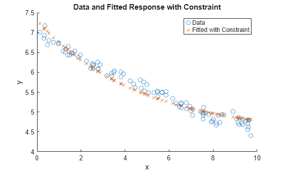
残差 res2 是残差 res 的两倍以上,而后者没有非线性约束。该结果表明,非线性约束使解远离无约束的最小值。
绘制有和没有非线性约束的解。
scatter(xdata,ydata)
hold on
scatter(xdata,fitfun(sol,xdata),"x")
hold off
xlabel("x")
ylabel("y")
legend("Data","Fitted")
title("Data and Fitted Response, No Constraint")
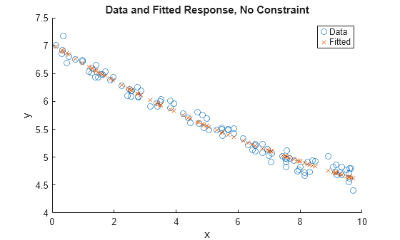
figure
scatter(xdata,ydata)
hold on
scatter(xdata,fitfun(sol2,xdata),"x")
hold off
xlabel("x")
ylabel("y")
legend("Data","Fitted with Constraint")
title("Data and Fitted Response with Constraint")
输入参数
名称-值参数
输出参量
详细信息
版本历史记录
在 R2023b 中推出