Dynamically Adapt PI Gains Online Using Reinforcement Learning

R2026b

This example uses:

This example shows how to use reinforcement learning (RL) to continually adapt the proportional-integral (PI) gains of a PID controller depending on the plant current operating condition.

Specifically, this example shows the third of three common approaches to using RL for proportional-integral (PI) parameter tuning. The three approaches are described in Tuning PI Gains Using Reinforcement Learning and are as follows:

1) Single Fixed Gains Across Multiple Operating Points, see Tune Fixed PI Gains Using Reinforcement Learning.

2) Fixed Set of Gains per Initial Condition, see Schedule PI Gains Per Initial Condition Using Reinforcement Learning.

3) Dynamically Adapt Gains Online (this example).

With the approach shown in this example, the goal is to dynamically adapt, during plant operation, the PI gains of a PID controller. This approach is adequate in a scenario in which the plant conditions affect the plant behavior and can also substantially change during operation. Here, you expect the controller to work only if the PI gains keep on adapting to the current plant operating conditions.

For more information, see Tuning PI Gains Using Reinforcement Learning.

Open Simulink Model

The plant model in this example is a water tank, implemented in the Simulink® model watertankLQG.slx, which is included as a supporting file. The model includes a PI controller that maintains the water level in the tank at a reference value.

Open the model.

WaterTankModel = 'watertankLQG';
open_system(WaterTankModel)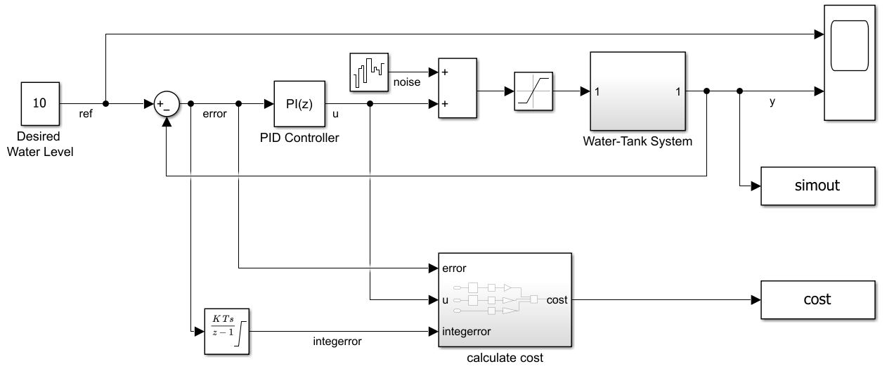

watertankLQG Simulink model with PID controller, water tank system, and cost calculation

The two To Workspace blocks simout and cost save the water level signal y and the cost signal, respectively, to the MATLAB® workspace, for later inspection. The model includes process noise with variance $E (n^{2} (t)) = 0.01$ .

The PID controller block used in the model implements a discrete-time PI controller. To maintain the water level $y$ at the target value while minimizing control action u, the PI gains of the PID controller are chosen, using the Control System Tuner (CST), to minimize the cumulative cost. This cumulative cost corresponds to the following linear quadratic Gaussian (LQG) criterion:

$J_{LQG} = \lim_{T \Rightarrow \infty} E (\frac{1}{T} \sum_{t = 0}^{T} ({(Href - y (t))}^{2} + 0.01 u^{2} (t) + 0.0001 {(\sum_{k = 0}^{t} Ts (Href - y (k)))}^{2}))$

Here, $J_{L Q G}$ is the cumulative cost, $Href$ is the desired water level, T is the number of time steps, and $Ts$ is the sample time.

The term $\sum_{k = 0}^{t} Ts (Href - y (k))$ is the discrete-time integral of the error, which is also calculated inside the PID controller block and fed back as a part of the control signal through the integral gain Ki to keep the steady-state error close to zero. For consistency with the examples that show other approaches, and with the PI controller designed using CST, this example uses $J_{L Q G}$ as cost to minimize. For more information on using Control System Tuner, see Tune a Control System Using Control System Tuner (Simulink Control Design).

To simulate the controller in this model, you must specify the simulation time Tf and the controller sample time Ts, in seconds.

Ts = 1;
Tf = 100;

For more information about the water tank model, see watertank Simulink Model (Simulink Control Design).

Specify Random Number Stream Seed and Algorithm for Reproducibility

The example code might involve computation of random numbers at several stages. Fixing the random number stream at the beginning of some sections in the example code preserves the random number sequence in the section every time you run it, which is a necessary condition to reproduce the results. For more information, see Results Reproducibility.

Specify the random number stream with the seed 0 and random number algorithm Mersenne Twister. For more information on controlling the seed used for random number generation, see rng.

previousRngState = rng(0,"twister");

The output previousRngState is a structure that contains information about the previous state of the stream. You will restore the state at the end of the example.

Online Adaptive PI Gain Adjustment

Use the approach in this example to continuously adapt PI gains to improve performance. Here, the RL agent takes as input an observation that includes both the error and the plant operating condition, and outputs the PI gains that corresponds to that pair of error and operating condition. The operating condition, which in this example consists in a vector containing both the reference and the initial water heights, is also called the context.

Key implementation details:

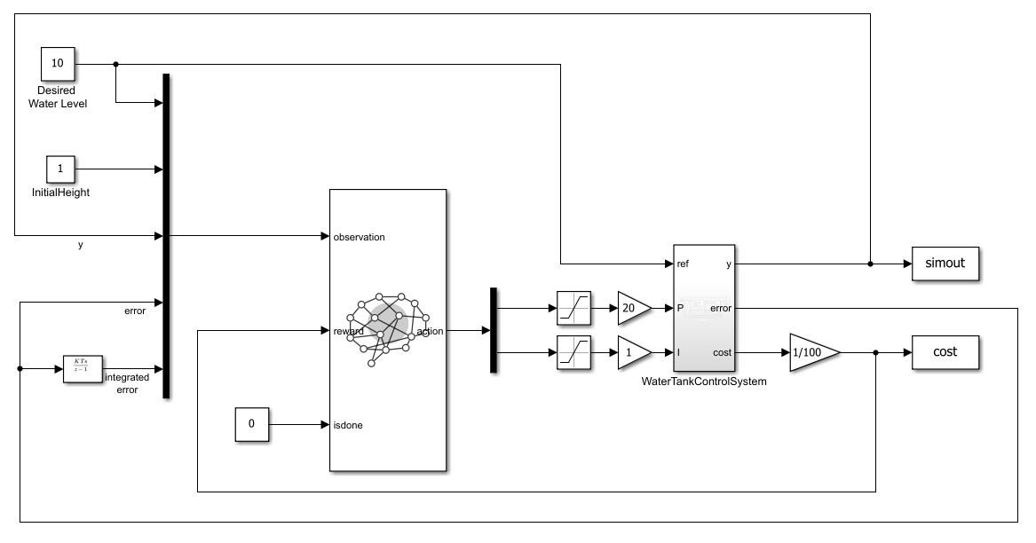
This approach uses a Simulink® environment that relies on the model rlWatertankPITuningUseCase3.slx, which is included as a supporting file.
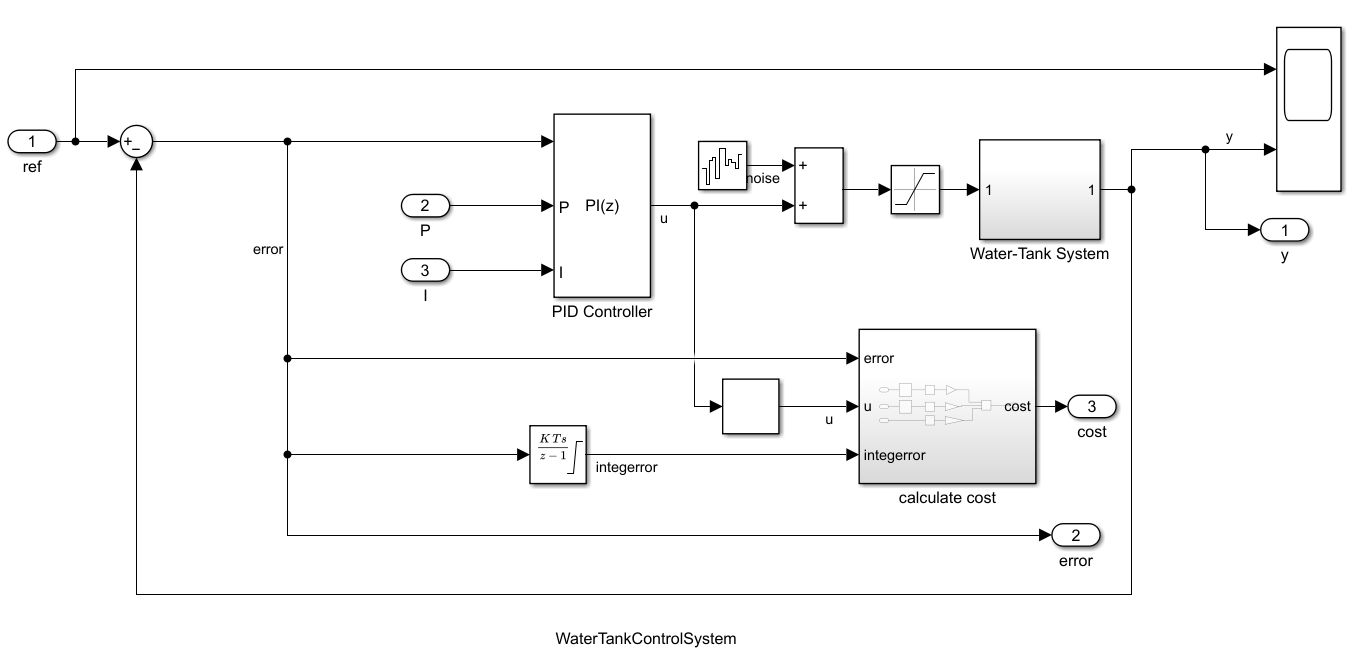
The WaterTankControlSystem subsystem contains a PI controller and a water tank model. It is a modified version of the watertankLQG.slx model for this problem. Given the reference water level and the PI gains, it controls the water tank model and then outputs the current water level, the error between the reference water level, and the current water level, the output of the PI controller, and the LQG cost.
As in the first approach, define the reward function for the RL agent as the negative of the scaled LQG cost, that is: $Reward = - 0.01 ({(Href - h (t))}^{2} + 0.01 u^{2} (t) + 0.0001 {(\sum_{k = 0}^{t} Ts (Href - y (k)))}^{2})$ .
The RL agent outputs a normalized action between zero and one and then the environment scales the action to the appropriate values of Kp and Ki, which have a different range of potential optimal gains.

The rlWatertankPITuningUseCase3 model is shown below:

rlWatertankPITuningUseCase3 model with RL Agent block connected to WaterTankControlSystem

The WaterTankControlSystem subsystem is shown below:

WaterTankControlSystem subsystem with PI controller, water tank, noise, and cost calculation

Create Environment Object

To reproduce the results of this section, specify the seed and algorithm used for random number generation.

rng(0,"twister");

Open the Simulink model.

mdl = 'rlWatertankPITuningUseCase3';
open_system(mdl)

Define the observation specification obsInfo. The observation contains the reference, initial, and current water levels, as well as the error and its integral.

obsInfo = rlNumericSpec([5 1]);

Define the action specification actInfo.

actInfo = rlNumericSpec([2 1]);
actInfo.LowerLimit = 0;
actInfo.UpperLimit = 1;

Build the environment object.

env3 = rlSimulinkEnv(mdl,[mdl '/RL Agent'],obsInfo,actInfo);

Set a custom reset function that randomizes the reference value and the initial state of the model.

env3.ResetFcn = @(in)localResetFcn3(in,mdl);

Create RL Agent

To reproduce the results of this section, specify the seed and algorithm used for random number generation.

rng(0,"twister");

Create a default twin-delayed deep deterministic (TD3) agent.

iniOpts = rlAgentInitializationOptions("NumHiddenUnit",128);
agent3 = rlTD3Agent(obsInfo,actInfo,iniOpts);

Set the agent hyperparameters using dot notation. Here, agent2.AgentOptions is an rlTD3AgentOptions option object.

Set the agent to use the controller sample time Ts.
Set a relatively small learning rate for both actor and critic to promote convergence.
Set a gradient threshold for both actor and critic to avoid drastic updates.
Set the learning frequency to -1. This value means that the agent updates at the end of each episode.
Set the max number of minibatches per epoch to 30 to reduce the number of gradient step updates for each learning iteration.
Set the mini-batch size to 128 experience samples to reduce the variance when computing gradients.
Set the experience buffer length to 1e6 to store a diverse set of experiences.
Set the standard deviation decay rate to 1e-5 to promote convergence after the exploration phase.
Set the standard deviation of the target policy smooth model to 0.1 to promote exploitation of actions with high Q-value estimates.

agent3.SampleTime = Ts;
agent3.AgentOptions.ActorOptimizerOptions.LearnRate = 5e-4;
agent3.AgentOptions.ActorOptimizerOptions.GradientThreshold = 1;
agent3.AgentOptions.CriticOptimizerOptions(1).LearnRate = 5e-4;
agent3.AgentOptions.CriticOptimizerOptions(1).GradientThreshold = 1;
agent3.AgentOptions.CriticOptimizerOptions(2).LearnRate = 5e-4;
agent3.AgentOptions.CriticOptimizerOptions(2).GradientThreshold = 1;
agent3.AgentOptions.LearningFrequency = -1;
agent3.AgentOptions.MaxMiniBatchPerEpoch = 30;
agent3.AgentOptions.MiniBatchSize = 128;
agent3.AgentOptions.ExperienceBufferLength = 1e6;
agent3.AgentOptions.ExplorationModel.StandardDeviationDecayRate = 1e-5;
agent3.AgentOptions.ExplorationModel.StandardDeviationMin = 0.1;
agent3.AgentOptions.TargetPolicySmoothModel.StandardDeviation=0.1;

Train RL Agent

To reproduce the results of this section, specify the seed and algorithm used for random number generation.

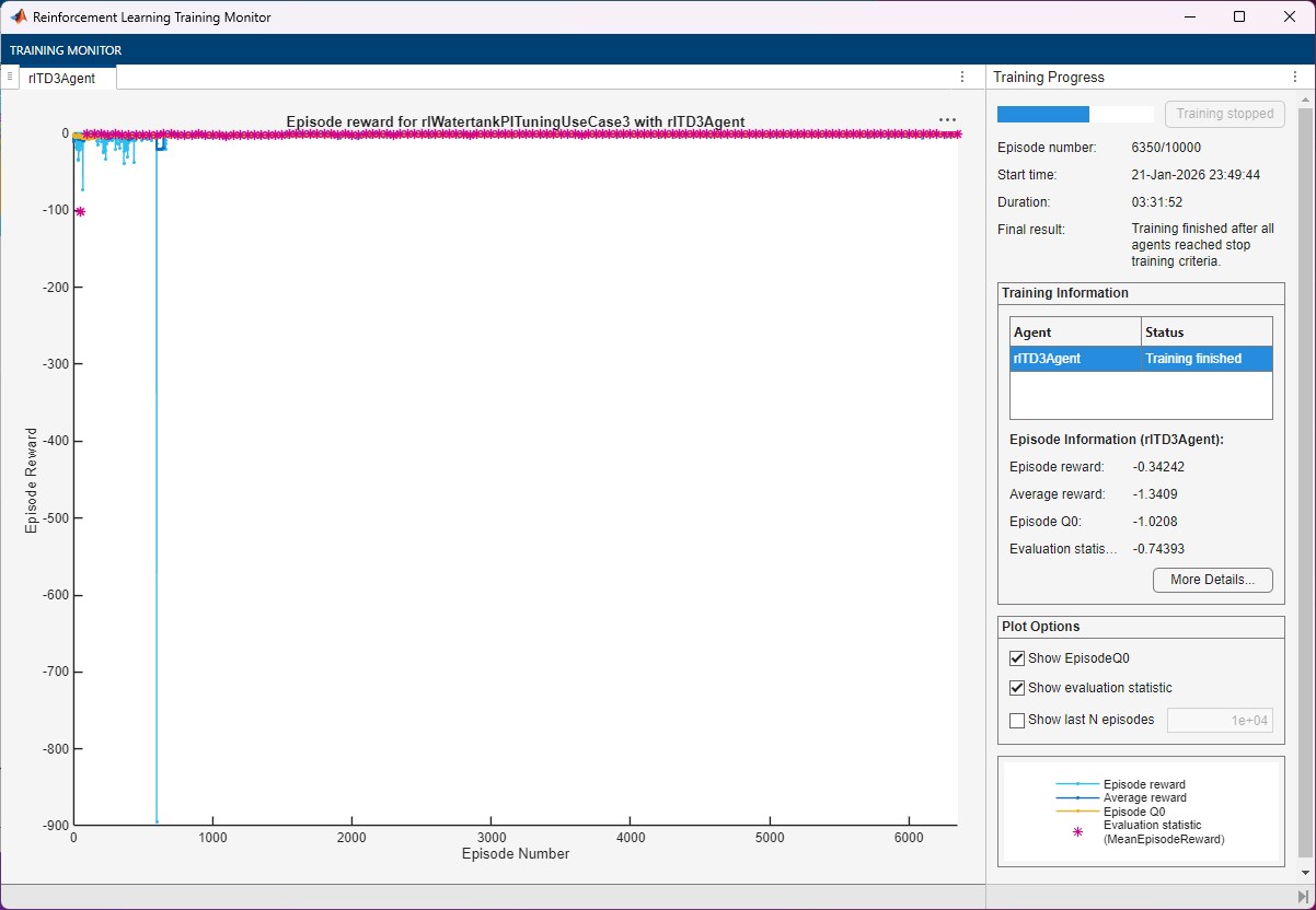
rng(0,"twister");

Create an evaluator object that evaluates the performance of the agent over 10 evaluation episodes every 50 training episodes, using the random seeds 1 to 10. The seeds randomize the initial conditions. The evaluation score is the average cumulative reward over the 10 evaluation episodes.

evl3 = rlEvaluator("NumEpisodes",10,"EvaluationFrequency",50,"RandomSeeds",1:10);

To train the agent, first specify the following training options.

Run each training for a maximum of 10000 episodes, with each episode lasting a maximum of 100 time steps.
Display the training progress in the Reinforcement Learning Training Monitor (set the Plots option to "training-progress") and disable the command-line display (set the Verbose option to false).
Stop the training when the evaluation score reaches -0.75. When the evaluation score reaches this level, the agent is capable of maintaining the water level at the reference value.

maxepisodes = 10000;
maxsteps = ceil(Tf/Ts);
trainOpts3 = rlTrainingOptions(...
    MaxEpisodes=maxepisodes, ...
    MaxStepsPerEpisode=maxsteps, ...
    ScoreAveragingWindowLength=50, ...
    SimulationStorageType = "none", ...
    Verbose=false, ...
    Plots="training-progress",...
    StopTrainingCriteria="EvaluationStatistic",...
    StopTrainingValue=-0.75);

Train the agent by using the train function. Training this agent is a computationally intensive process. To save time, load a pretrained agent by setting doTraining to false. To train the agent yourself, set doTraining to true.

doTraining = false;
if doTraining
    % Train the agent.
    trainingStats3 = train(agent3,env3,trainOpts3,Evaluator=evl3);
else
    % Load pretrained agent for the example.
    load("WaterTankPITuningTD3AgentUseCase3.mat","agent3");
end

Training Monitor showing episode reward converging near zero over 6350 episodes

Validate Trained Agent

To reproduce the results of this section, specify the seed and algorithm used for random number generation.

rng(0,"twister");

By default, the agent uses a greedy (hence deterministic) policy in simulation. If needed, you can use the exploratory policy instead, by setting the UseExplorationPolicy agent property to true.

To validate the trained agent, simulate it within the environment for maxsteps steps. For more information on agent simulation, see sim.

simOpts = rlSimulationOptions(MaxSteps=maxsteps);
experiences = sim(env3,agent3,simOpts);

Show the cumulative reward obtained during the simulation episode.

sum(experiences.Reward.Data)

ans = 
-1.3635

The cumulative reward is close to the value obtained in the last training episodes, which suggests that the policy is able to stabilize the water level at the desired value.

Analyze Controller Performance

In this section, you return to the original WaterTankModel Simulink model and apply the policy obtained using RL.

To reproduce the results of this section, specify the seed and algorithm used for random number generation.

rng(0,"twister");

Validate the trained agent against the model by simulation and extract the step response information and LQG cost.

load_system(mdl);
% Set initial condition.
refWaterLevel = 10;
initialWaterLevel = 1;
randomSeed = 1;
% Create simulink.simulationInput object to store temporary changes to the model.
simIn = Simulink.SimulationInput(mdl);
refBlk = sprintf([mdl '/Desired \nWater Level']);
simIn = setBlockParameter(simIn,refBlk,'Value',num2str(refWaterLevel));
initBlk = [mdl '/WaterTankControlSystem/Water-Tank System/H'];
simIn = setBlockParameter(simIn,initBlk,'InitialCondition',num2str(initialWaterLevel));
initBlk2 = [mdl '/InitialWaterLevel'];
simIn = setBlockParameter(simIn,initBlk2,'Value',num2str(initialWaterLevel));

Simulate the model.

simResults = sim(simIn);
rlStep3 = simResults.simout;
rlCost3 = simResults.cost;

A linearization-based stability analysis of this adaptive PI controller might not accurately reflect the stability of the overall system. Since the controller's parameters can change over time, the linearized model at a single snapshot (e.g., at t = 50 seconds) might not represent the system behavior at other times. Instead, to analyze the stability of the system at each time step, use the localStabilityAnalysis3 function, which is defined at the end of this example. Note that, however, these margins are still local to each snapshot and do not guarantee global stability of the full time-varying closed loop.

blockIn  = [mdl '/WaterTankControlSystem/Sum1'];
blockOut = [mdl '/WaterTankControlSystem/Water-Tank System'];
blockLoopBreak1 = [mdl '/WaterTankControlSystem/P'];
blockLoopBreak2 = [mdl '/WaterTankControlSystem/I'];
rlStabilityMargin3 = localStabilityAnalysis3(mdl,...
                                            blockIn,blockOut,...
                                            blockLoopBreak1,...
                                            blockLoopBreak2,...
                                            Ts,Tf);

Find the indices at which the system is unstable. The unstableModelIndex variable is empty if the system remains stable at all times.

unstableModelIndex = find(~[rlStabilityMargin3.Stable])

unstableModelIndex =

  1×0 empty double row vector

Compute the LQG cost.

rlCumulativeCost3  = -sum(rlCost3.Data)

rlCumulativeCost3 = 
1.4570

To analyze the step response, use the stepinfo (Control System Toolbox) function.

rlStepInfo3 = stepinfo(rlStep3.Data,rlStep3.Time);

Create a table with the most relevant time response data.

stepInfoTable = struct2table(rlStepInfo3);
stepInfoTable = removevars(stepInfoTable,{'SettlingMin', ...
    'TransientTime','SettlingMax','Undershoot','PeakTime'});
stepInfoTable.Properties.RowNames = {'RL3 Adaptive'};

Display the table.

stepInfoTable

stepInfoTable = 1×4 table
                    RiseTime    SettlingTime    Overshoot    Peak 
                    ________    ____________    _________    _____

    RL3 Adaptive     3.0607        13.361        10.915      11.12

Analyze the stability at 50 seconds into the simulation.

stabilityMarginTable = struct2table( ...
    [rlStabilityMargin3(51)]);
stabilityMarginTable = removevars(stabilityMarginTable,{...
    'GMFrequency','PMFrequency','DelayMargin','DMFrequency'});
stabilityMarginTable.Properties.RowNames = {'RL3 Adaptive'};
stabilityMarginTable

stabilityMarginTable = 1×3 table
                    GainMargin    PhaseMargin    Stable
                    __________    ___________    ______

    RL3 Adaptive      3.1778        43.009       true

The controller at the selected time instant has ample gain and phase margins.

Restore the random number stream using the information stored in previousRngState.

rng(previousRngState);

Local Functions

localResetFcn3 function randomizes the reference signal and the initial water level.

function in = localResetFcn3(in,mdl)
    % Randomize disturbance signal.
    randomSeed = randi(10000);
    noiseBlk = sprintf([mdl '/WaterTankControlSystem/Band-Limited\nWhite Noise/']);
    in = setBlockParameter(in,noiseBlk,'Seed',num2str(randomSeed));

    % Randomize reference signal.
    hRef = 10 + 4*(rand-0.5);
    hRefBlk = sprintf([mdl '/Desired \nWater Level']);
    in = setBlockParameter(in,hRefBlk,'Value',num2str(hRef));

    % Randomize initial water level.
    hInit = 2*rand;
    hInitBlk = [mdl '/WaterTankControlSystem/Water-Tank System/H'];
    in = setBlockParameter(in,hInitBlk,'InitialCondition',num2str(hInit));
    hInitBlk2 = [mdl '/InitialWaterLevel'];
    in = setBlockParameter(in,hInitBlk2,'Value',num2str(hInit));
end

The localStabilityAnalysis3 function computes the stability margins by linearizing mdl at each time step.

function margin = localStabilityAnalysis3(mdl,...
                                          blockIn,blockOut,...
                                          blockLoopBreak1,...
                                          blockLoopBreak2,...
                                          Ts,Tf)
    set_param(mdl,"FastRestart","off")
    io(1) = linio(blockIn,1,'input');    
    io(2) = linio(blockOut,1,'openoutput');
    io(3) = linio(blockLoopBreak1,1,'loopbreak');
    io(4) = linio(blockLoopBreak2,1,'loopbreak');            
    op = 0:Ts:Tf; 
    linsys = linearize(mdl,io,op);
    margin = allmargin(linsys);
end

Dynamically Adapt PI Gains Online Using Reinforcement Learning

Open Simulink Model

Specify Random Number Stream Seed and Algorithm for Reproducibility

Online Adaptive PI Gain Adjustment

Create Environment Object

Create RL Agent

Train RL Agent

Validate Trained Agent

Analyze Controller Performance

Local Functions

See Also

Functions

Objects

Topics