Schedule PI Gains Per Initial Condition Using Reinforcement Learning

R2026b

This example uses:

This example shows how to use reinforcement learning (RL) to find a mapping between a plant initial condition and a respective single set of proportional-integral (PI) gains of a PID controller.

Specifically, this example shows the second of three common approaches to using RL for proportional-integral (PI) parameter tuning. The three approaches are described in Tuning PI Gains Using Reinforcement Learning and are as follows:

1) Single Fixed Gains Across Multiple Operating Points, see Tune Fixed PI Gains Using Reinforcement Learning.

2) Fixed Set of Gains per Initial Condition, (this example).

3) Online Dynamically Adaptive Gains, see Dynamically Adapt PI Gains Online Using Reinforcement Learning.

With the approach shown in this example, the goal is to find a mapping from each possible initial condition to its corresponding PI gains. This approach is adequate in a scenario in which the plant conditions substantially affect the plant behavior, but they do not change during plant operation. In other words, in this scenario, you don't expect that a single set of gains can always work, but you think that, given the plant initial condition, there exist a corresponding fixed set of gains that can drive the plant towards the desired behavior.

For more information, see Tuning PI Gains Using Reinforcement Learning.

Open Simulink Model

The plant model in this example is a water tank, implemented in the Simulink® model watertankLQG.slx, which is included as a supporting file. The model includes a PI controller that maintains the water level in the tank at a reference value.

Open the model.

WaterTankModel = 'watertankLQG'

WaterTankModel = 
'watertankLQG'

open_system(WaterTankModel)

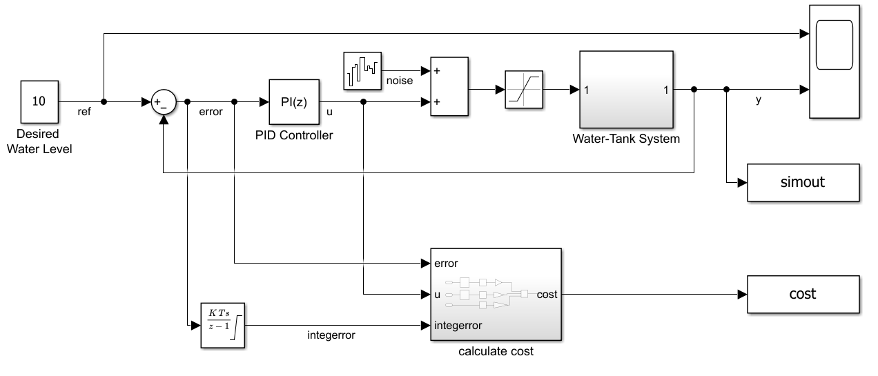
Simulink model of the water tank environment with a discrete PI controller, process noise, and cost calculation subsystem

The two To Workspace blocks simout and cost save the water level signal y and the cost signal, respectively, to the MATLAB® workspace, for later inspection. The model includes process noise with variance $E (n^{2} (t)) = 0.01$ .

The PID controller block used in the model implements a discrete-time PI controller. To maintain the water level $y$ at the target value while minimizing control action u, the PI gains of the PID controller are chosen, using the Control System Tuner (CST), to minimize the cumulative cost. This cumulative cost corresponds to the following linear quadratic Gaussian (LQG) criterion:

$J_{LQG} = \lim_{T \Rightarrow \infty} E (\frac{1}{T} \sum_{t = 0}^{T} ({(Href - y (t))}^{2} + 0.01 u^{2} (t) + 0.0001 {(\sum_{k = 0}^{t} Ts (Href - y (k)))}^{2}))$

Here, $J_{L Q G}$ is the cumulative cost, $Href$ is the desired water level, T is the number of time steps, and $Ts$ is the sample time.

The term $\sum_{k = 0}^{t} Ts (Href - y (k))$ is the discrete-time integral of the error, which is also calculated inside the PID controller block and fed back as a part of the control signal through the integral gain Ki to keep the steady-state error close to zero. For consistency with the examples that show other approaches, and with the PI controller designed using CST, this example uses $J_{L Q G}$ as cost to minimize. For more information on using Control System Tuner, see Tune a Control System Using Control System Tuner (Simulink Control Design).

To simulate the controller in this model, you must specify the simulation time Tf and the controller sample time Ts, in seconds.

Ts = 1;
Tf = 100;

For more information about the water tank model, see watertank Simulink Model (Simulink Control Design).

Specify Random Number Stream Seed and Algorithm for Reproducibility

The example code might involve computation of random numbers at several stages. Fixing the random number stream at the beginning of some sections in the example code preserves the random number sequence in the section every time you run it, which is a necessary condition to reproduce the results. For more information, see Results Reproducibility.

Specify the random number stream with the seed 0 and random number algorithm Mersenne Twister. For more information on controlling the seed used for random number generation, see rng.

previousRngState = rng(0,"twister");

The output previousRngState is a structure that contains information about the previous state of the stream. You will restore the state at the end of the example.

Contextual Bandits Approach to Gain Scheduling

In this example, you use a contextual bandit approach to automatically tune a set of PI gains for a corresponding water tank condition. Here, the RL agent takes as input an observation that indicates a plant operating condition and outputs the PI gains that corresponds to that operating condition. The operating condition, which in this example consists in a vector containing both the reference and the initial water heights, is also called the context.

In this approach one 100-seconds simulation corresponds to a single reinforcement learning environment step. The agent is trained over 2000 episodes, each one consisting of 100 environment steps. Therefore, during training, 100 independent Simulink simulations (each lasting 100 seconds) are executed within a single episode.

Key implementation details:

This approach uses a MATLAB environment object (not a Simulink-based environment as in other approaches). You create the environment object using the constructor function in the class WaterTankPITunerContextualBanditsEnv, which is included as a supporting file. This environment implements a contextual bandit workflow. Within each environment step, the environment takes the action (one couple of PI gains) from the agent, runs a single Simulink simulation, collects the cumulative reward which is used for learning, and then immediately creates a new random context (reference and initial water levels) for the next simulation. The action chosen for the current environment step does not influence future values of the context or future rewards. For an example on contextual bandits, see Train Reinforcement Learning Agent for Simple Contextual Bandit Problem.
At each environment step, the environment computes the reward using the output from the Simulink simulation. Note that this is different from the first approach, in which the reward was computed directly in the closed-loop simulink model. In this example, the weighted sum of the total LQG cost, the overshoot time ( $t_{o v e r s h o o t}$ ), and the settling time ( $t_{s e t t l i n g t i m e}$ ), is used as the reward: $Reward = - w_{1} \sum_{t}^{T} ({(Href - y (t))}^{2} + 0.01 u^{2} (t) + 0.0001 {(\sum_{k = 0}^{t} Ts (Href - y (k)))}^{2}) - w_{2} t_{o v e r s h o o t} - w_{3} t_{s e t t l i n g t i m e}$ , with weights $w_{1} = 0.01, w_{2} = 0.5, w_{3} = 0.5$ . This reward formulation differs from the one used in the first approach, highlighting the flexibility of the reward function in the contextual bandit framework.
Usually, contextual bandits involve only one step (single bandit simulation) per episode. In this example, to reduce training time, multiple independent bandit simulations are performed within a single episode, eliminating the overhead between episodes. There is no state carried over from one environment step to the next, because the environment samples the new context randomly at each environment step. Therefore, the environment keeps the IsDone signal to false. The number of environment steps in each episode is controlled only by the MaxStepsPerEpisode property of the rlTrainingOptions object that you provide as input to the train function.
The RL agent is configured with a discount factor of zero (DiscountFactor=0) because there is no temporal dependence across steps. Each environment step is independent and only the immediate reward matters.
The RL agent outputs a normalized action between zero and one and then the environment scales the action to the appropriate values of Kp and Ki, which have a different range of potential optimal gains.

Display the environment class file.

type WaterTankPITunerContextualBanditsEnv

classdef WaterTankPITunerContextualBanditsEnv < rl.env.MATLABEnvironment
    % WaterTankPITunerContextualBanditsEnv: The environment is a water tank environment where the
    % goal of this control system is to maintain the level of water in a tank to
    % match a reference value.
    %
    % Contextual bandit usage and training guidance:
    % - This environment implements a contextual bandit workflow to reduce training
    %   time: each step runs a single Simulink trial and immediately
    %   samples a new random context (reference, initial water level).
    % - Episodes do not terminate automatically (IsDone is always false) so that
    %   many independent bandit trials can occur within one episode.
    % - Configure the agent with discount factor = 0, because there
    %   is no temporal credit assignment across steps; each step is independent.
    
    % Copyright 2026 The MathWorks, Inc.

    properties
        % Initial observation
        InitialObservation =[10;1];
        % Desired water level 
        HRef = 10;
        % Initial water level
        HInit = 1;
        % Random seed for disturbance
        DisturbanceRandomSeed = 123;
        % Kp scaling
        KpScale = 20;
        % Ki scaling
        KiScale = 1;        
        % Weights for reward
        WeightCost = 1/100;
        WeightOvershoot = 0.5;
        WeightSettlingTime = 0.5;
    end

    properties (SetAccess = private)
        % Simulink model
        Model
        Ts = 1
        Tf = 100
    end

    properties (Access = private)
        % SimulationInput template for reuse
        SimInputTemplate
    end

    methods              
        function this = WaterTankPITunerContextualBanditsEnv(Model, Ts, Tf)
            arguments
                Model
                Ts (1,1) = 1
                Tf (1,1) = 100
            end
            % Define the observation specification obsInfo
            observationInfo = rlNumericSpec([2 1]);            
            observationInfo.Description = 'Desired water level and current water level';

            % Define action Info
            actionInfo = rlNumericSpec([2 1]);            
            actionInfo.Description = 'Kp and Ki';
            actionInfo.LowerLimit = 0;
            actionInfo.UpperLimit = 1;

            this = this@rl.env.MATLABEnvironment(observationInfo,actionInfo);
            this.Model = Model;

            % Load the model if not loaded
            if ~bdIsLoaded(Model)
                load_system(Model);
            end

            % Build a SimulationInput template for reuse
            this.Ts = Ts;
            this.Tf = Tf;
            this.SimInputTemplate = Simulink.SimulationInput(Model);
            this.SimInputTemplate = setVariable(this.SimInputTemplate, 'Ts', this.Ts);
            this.SimInputTemplate = setVariable(this.SimInputTemplate, 'Tf', this.Tf);  
        end
        
        function [Observation,Reward,IsDone,Info] = step(this,Action)

            if iscell(Action)
                Action = Action{1};
            end
            Action = max(min(Action,1),0);
            % Prepare SimulationInput from template and set parameters via cached handles
            simin = this.SimInputTemplate;            
            simin = setBlockParameter(simin, [this.Model '/PID Controller'],    'P', num2str(Action(1) * this.KpScale));
            simin = setBlockParameter(simin, [this.Model '/PID Controller'],    'I', num2str(Action(2) * this.KiScale));
            simin = setBlockParameter(simin, [this.Model '/' sprintf('Desired \nWater Level')],   'Value', num2str(this.HRef));
            simin = setBlockParameter(simin, [this.Model '/Water-Tank System/H'], 'InitialCondition', num2str(this.HInit));
            simin = setBlockParameter(simin, [this.Model '/' sprintf('Band-Limited\nWhite Noise')], 'Seed', num2str(this.DisturbanceRandomSeed));

            % Run the simulation
            out = sim(simin,UseFastRestart="on");

            % Compute reward
            Reward = getReward(this, out);

            % Contextual bandit training pattern to reduce training time:
            % 1) Immediately sample a new context by calling reset() after each
            %    simulation trial. The new context becomes the next Observation
            %    returned to the agent.
            % 2) Keep IsDone = false so a single episode can contain many
            %    independent bandit trials.
            this.InitialObservation = reset(this);            
            Observation = this.InitialObservation;                      
            IsDone = false;

            % Info
            Info = [];
        end
        
        function reward = getReward(this, out)            
            % Compute LQG cost
            cost = sum(abs(out.cost.Data));

            % Compute overshoot and settling time
            currentWaterLevelStep = out.simout;
            stepInfoResult = stepinfo(currentWaterLevelStep.Data,currentWaterLevelStep.Time);                        
            overshoot               = stepInfoResult.Overshoot;
            settlingTime            = stepInfoResult.SettlingTime;

            % Saturate overshoot
            overshoot = min(max(overshoot,-20),20);
            % Saturate settling time
            settlingTime = min(max(settlingTime,-100),100);
            
            % Compute the total cost
            totalCost =   this.WeightCost * cost ...
                   + this.WeightOvershoot * overshoot ...
                   + this.WeightSettlingTime * settlingTime;
            reward = -totalCost;                             
        end

        % Reset environment to initial state and output initial observation
        function InitialObservation = reset(this)
            % Randomize seed for disturbance signal
            this.DisturbanceRandomSeed = randi(10000);

            % Randomize reference signal
            this.HRef = 10 + 4*(rand-0.5);

            % Randomize initial water level
            this.HInit = 2*rand;

            InitialObservation = [this.HRef;this.HInit];                  
            this.InitialObservation = InitialObservation;            
        end
    end
end

Contextual Bandits Objective Clarification: Simple Regret over Cumulative Regret

In the field of contextual bandits, minimizing cumulative regret is often the main objective. Cumulative regret is the difference between the cumulative reward that the agent actually receives and the cumulative reward that it would have received by always choosing the best possible action in hindsight. This criteria makes no distinction between the training phase (during which exploration is required) and the deployment phase, because it adds up all the losses incurred during the learning process.

However, in this example, our focus is on minimizing simple regret. Simple regret is the difference between the single reward that the agent actually receives for the recommended action and the single reward that it would have received by recommending the best possible action in hindsight. Here, the goal is for the agent to optimize its performance during the evaluation phase, without considering the cost incurred during training.

Create Environment Object

To reproduce the results of this section, specify the seed and algorithm used for random number generation.

rng(0,"twister");

To construct the environment, provide the water take model as an input argument to the WaterTankPITunerContextualBanditsEnv function.

% Simulink model
load_system(WaterTankModel)
set_param(WaterTankModel,"FastRestart","on")
% Construct MATLAB environment.
env2 = WaterTankPITunerContextualBanditsEnv(WaterTankModel,Ts,Tf);

The environment constructor function internally defines the observation and action specifications. Get the specifications from the environment.

obsInfo = getObservationInfo(env2)

obsInfo = 
  rlNumericSpec with properties:

     LowerLimit: -Inf
     UpperLimit: Inf
           Name: [0×0 string]
    Description: "Desired water level and current water level"
      Dimension: [2 1]
       DataType: "double"

Get the action specification from the environment.

actInfo = getActionInfo(env2)

actInfo = 
  rlNumericSpec with properties:

     LowerLimit: 0
     UpperLimit: 1
           Name: [0×0 string]
    Description: "Kp and Ki"
      Dimension: [2 1]
       DataType: "double"

The KpScale environment property scales the action from [0,1] to the range of potential optimal gains for Kp. The KiScale environment property scales the action from [0,1] to the range of potential optimal gains for Ki.

env2.KpScale = 20;
env2.KiScale = 1;

The environment uses three weights to compute the reward, which is the weighted sum of the LQG cost, the overshoot time, and the settling time.

env2.WeightCost         = 0.01;
env2.WeightOvershoot    = 0.5;
env2.WeightSettlingTime = 0.5;

Create RL Agent

To reproduce the results of this section, specify the seed and algorithm used for random number generation.

rng(0,"twister");

Create a default deep deterministic policy gradient (DDPG) agent. The DDPG agent uses a single critic network to learn the optimal policy, which is sufficient for this problem because the critic only needs to estimate the immediate reward and does not suffer from overestimation.

initOptions = rlAgentInitializationOptions("NumHiddenUnit",128);
agent2 = rlDDPGAgent(obsInfo,actInfo,initOptions);

Set the agent hyperparameters using dot notation. Here, agent2.AgentOptions is an rlDDPGAgentOptions option object.

Set DiscountFactor to 0. In the contextual bandit setting, the agent considers only the immediate reward, so future rewards (which are unrelated to the current action) can be completely discounted.
Use Gaussian noise is for exploration instead of Ornstein-Uhlenbeck (OU) noise, because the contextual bandit setting does not require temporally correlated noise.
Set TargetSmoothFactor and TargetUpdateFrequency to 1, so that the target actor and critic networks are always identical to the current (online) actor and critic networks. Typically, DDPG agents use target networks to stabilize training when learning from bootstrapped targets (that is using Q-value estimates of the next state-action pair). However, since there bootstrapping is not needed in a contextual bandits setting, the target networks can remain synchronized with the current networks at all times.
Set the learning frequency to -1. This value means that the agent updates at the end of each episode.
Set a relatively small learning rate for both actor and critic to promote convergence.
Set a gradient threshold for both actor and critic to avoid drastic updates.
Set the standard deviation decay rate to 5e-5 to promote convergence after the exploration phase.
Set the mini-batch size to 128 experience samples to reduce the variance when computing gradients.
Set the max number of minibatches per epoch to 10 to reduce the number of gradient step updates for each learning iteration.
Set the number of warm start steps to 512 to ensure that learning takes place over a more diverse data set at the beginning of training.

agent2.AgentOptions.DiscountFactor = 0;
agent2.AgentOptions.NoiseOptions = rl.option.GaussianActionNoise;
agent2.AgentOptions.TargetSmoothFactor = 1;
agent2.AgentOptions.TargetUpdateFrequency = 1;
agent2.AgentOptions.NoiseOptions.StandardDeviationDecayRate = 5e-5;
agent2.AgentOptions.NoiseOptions.StandardDeviationMin = 0.1;
agent2.AgentOptions.ActorOptimizerOptions.LearnRate = 5e-4;
agent2.AgentOptions.ActorOptimizerOptions.GradientThreshold = 1;
agent2.AgentOptions.CriticOptimizerOptions.LearnRate = 5e-4;
agent2.AgentOptions.CriticOptimizerOptions.GradientThreshold = 1;
agent2.AgentOptions.LearningFrequency = -1;
agent2.AgentOptions.MaxMiniBatchPerEpoch = 10;
agent2.AgentOptions.MiniBatchSize = 128;
agent2.AgentOptions.NumWarmStartSteps = 512;

Train RL Agent

To reproduce the results of this section, specify the seed and algorithm used for random number generation.

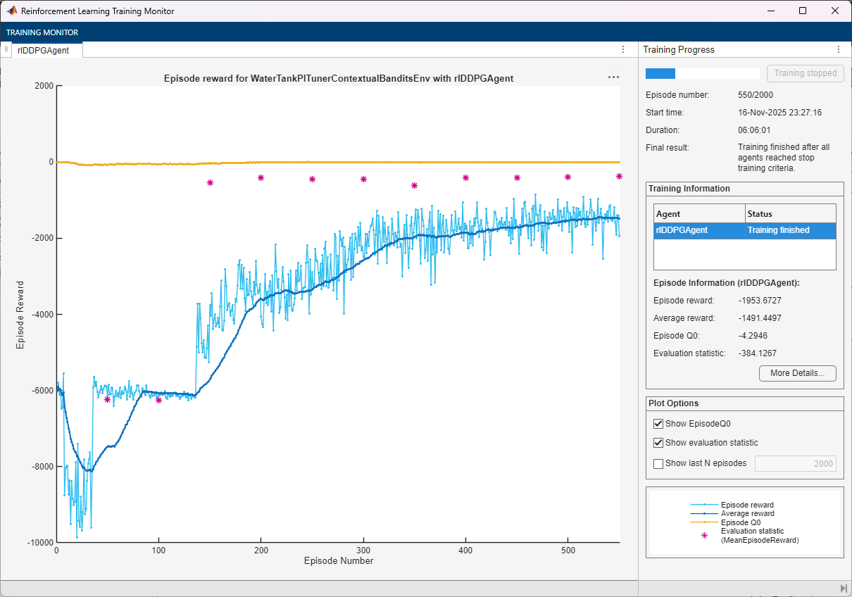
rng(0,"twister");

Create an evaluator object that evaluates the performance of the agent over 5 evaluation episodes every 50 training episodes, using the random seeds 1 to 5. The seeds randomize the initial conditions. The evaluation score is the average cumulative reward over the 5 evaluation episodes.

evl2 = rlEvaluator("NumEpisodes",5,"EvaluationFrequency",50,"RandomSeeds",1:5);

To train the agent, first specify the following training options.

Train the agent for a maximum of 2000 episodes, with each episode lasting a maximum of 100 environment steps. In this contextual bandit environment, each step runs a single independent simulation.
Display the training progress in the Reinforcement Learning Training Monitor (set the Plots option to "training-progress") and disable the command-line display (set the Verbose option to false).
Stop the training when the evaluation score reaches -390. When the evaluation score reaches this level, the agent is capable of maintaining the water level at the reference value.
Because WaterTankPITunerContextualBanditsEnv objects do not support parallel training, explicitly set the UseParallel property is set to "off". This is the default option.

maxepisodes = 2000;
trainOpts2 = rlTrainingOptions(...
    MaxEpisodes=maxepisodes, ...
    MaxStepsPerEpisode=100, ...
    ScoreAveragingWindowLength=50, ...
    UseParallel="off", ...
    Verbose=false, ...
    Plots="training-progress",...
    StopTrainingCriteria="EvaluationStatistic",...
    StopTrainingValue = -390);

Train the agent by using the train function. Training this agent is a computationally intensive process because each step runs a 100-seconds simulation, and it might take several hours to complete. To save time, load a pretrained agent by setting doTraining to false. To train the agent yourself, set doTraining to true.

doTraining = false;
if doTraining
    % Train the agent.
    trainingStats2 = train(agent2,env2,trainOpts2,Evaluator=evl2);
else
    % Load pretrained agent for the example.
    load("WaterTankPITuningDDPGAgentUseCase2.mat","agent2")
end

Training progress for the DDPG agent showing episode and average rewards improving over 550 episodes

Validate Trained Agent

To reproduce the results of this section, specify the seed and algorithm used for random number generation.

rng(0,"twister");

By default, the agent uses a greedy (hence deterministic) policy in simulation. If needed, you can use the exploratory policy instead, by setting the UseExplorationPolicy agent property to true.

To validate the trained agent, simulate it within the environment for maxsteps steps. For more information on agent simulation, see sim.

simOpts = rlSimulationOptions(MaxSteps=100);
experiences = sim(env2,agent2,simOpts);

Show the cumulative reward obtained during the simulation episode.

sum(experiences.Reward.Data)

ans = 
-383.7783

The cumulative reward is close to the value obtained in the last training episodes, which suggests that the policy is able to stabilize the water level at the desired value.

Analyze Controller Performance

In this section, you return to the original WaterTankModel Simulink model and apply the policy obtained using RL.

To reproduce the results of this section, specify the seed and algorithm used for random number generation.

rng(0,"twister");

Use the Simulink.SimulationInput (Simulink) object simIn to temporarily set the random seed for the noise, reference, and initial water levels in the respective blocks.

refWaterLevel = 10;
initialWaterLevel = 1;
randomSeed = 1;
simIn = Simulink.SimulationInput(WaterTankModel);
noiseBlk = sprintf([WaterTankModel '/Band-Limited\nWhite Noise/']);
simIn = setBlockParameter(simIn,noiseBlk,'Seed',num2str(randomSeed));
refBlk = sprintf([WaterTankModel '/Desired \nWater Level']);
simIn = setBlockParameter(simIn,refBlk,'Value',num2str(refWaterLevel));
initBlk = [WaterTankModel '/Water-Tank System/H'];
simIn = setBlockParameter(simIn,initBlk,'InitialCondition',num2str(initialWaterLevel));

Get Kp and Ki. These gains are the action recommended by the agent given the reference and initial water levels.

action = getAction(agent2,[refWaterLevel,initialWaterLevel]');
Kp = action{1}(1)*env2.KpScale

Kp = 
3.9052

Ki = action{1}(2)*env2.KiScale

Ki = 
2.9802e-08

Note that Ki is close to zero, which makes the controller essentially proportional.

In the PID controller block, set the P and I parameters to the PI gains obtained from the trained RL agent.

PIBlk = [WaterTankModel '/PID Controller'];
set_param([WaterTankModel '/PID Controller'],'P',num2str(Kp))
set_param([WaterTankModel '/PID Controller'],'I',num2str(Ki))

Use the Simulink sim function to simulate the water tank model with the applied temporary changes. The variable simResults that sim returns as output contains the fields simout and cost, which store the water level and cost recorded during the simulation. These fields are created by the two To Workspace blocks in the Simulink model.

simResults = sim(simIn);

Extract the step response information, the LQG cost signal, and calculate the open-loop stability margin. To compute the stability margin, use the localStabilityAnalysis function defined at the end of this example. The function returns a structure containing several stability margins, each one related to a snapshot of the system at a given time. Select a time of 50 seconds, which represents the midpoint of the 100-second simulation, when the system is expected to be near or at steady state.

rlStep2 = simResults.simout;
rlCost2 = simResults.cost;
blockIn  = [WaterTankModel '/PID Controller'];
blockOut = [WaterTankModel '/Water-Tank System'];
stabilityAnalysisTime = 50;
rlStabilityMargin2 = localStabilityAnalysis(WaterTankModel,...
                                            blockIn,...
                                            blockOut,...
                                            stabilityAnalysisTime);

To analyze the step response, use the stepinfo (Control System Toolbox) function.

rlStepInfo2 = stepinfo(rlStep2.Data,rlStep2.Time);
stepInfoTable = struct2table(rlStepInfo2);
stepInfoTable = removevars(stepInfoTable,{'SettlingMin', ...
    'TransientTime','SettlingMax','Undershoot','PeakTime'});
stepInfoTable.Properties.RowNames = {'RL2'};
stepInfoTable

stepInfoTable = 1×4 table
           RiseTime    SettlingTime    Overshoot     Peak 
           ________    ____________    _________    ______

    RL2     2.7637        3.3866        0.84997     9.7419

	Get insights using Copilot

Create a table with the most relevant stability margins.

stabilityMarginTable = struct2table(rlStabilityMargin2);
stabilityMarginTable = removevars(stabilityMarginTable,{...
    'GMFrequency','PMFrequency','DelayMargin','DMFrequency'});
stabilityMarginTable.Properties.RowNames = {'RL2'};
 stabilityMarginTable

stabilityMarginTable = 1×3 table
           GainMargin    PhaseMargin    Stable
           __________    ___________    ______

    RL2      8.0017        94.413       true  

	Get insights using Copilot

The controller has ample gain and phase margins.

Compute the cumulative LQG cost.

rlCumulativeCost2  = -sum(rlCost2.Data)

rlCumulativeCost2 = 
174.7657

The cumulative cost is comparable to that of of the first approach (see Tune Fixed PI Gains Using Reinforcement Learning).

Restore the random number stream, using the information stored in previousRngState.

rng(previousRngState);

Local Functions

The localStabilityAnalysis function computes stability margins by linearizing the closed-loop model at a specified time using loop-opening analysis points.

function margin = localStabilityAnalysis(mdl,blockIn,blockOut,time)
    set_param(mdl,"FastRestart","off")
    io(1) = linio(blockIn,1,'input');
    io(2) = linio(blockOut,1,'openoutput');
    op = operpoint(mdl);
    op.Time = time;
    linsys = linearize(mdl,io,op);
    margin =  allmargin(linsys);
end

Schedule PI Gains Per Initial Condition Using Reinforcement Learning

Open Simulink Model

Specify Random Number Stream Seed and Algorithm for Reproducibility

Contextual Bandits Approach to Gain Scheduling

Create Environment Object

Create RL Agent

Train RL Agent

Validate Trained Agent

Analyze Controller Performance

Local Functions

See Also

Functions

Objects

Topics